mag2exp.ltem.phase#
- mag2exp.ltem.phase(field, /, kcx=0.1, kcy=0.1)#
Calculation of the magnetic phase shift experienced by the electrons.
The Fourier transform of the magnetic phase shift is calculated using
\[\widetilde{\phi}_m (k_x,k_y) = \frac {i e \mu_0 k_\perp^2}{h} \frac{\left[ \widetilde{\bf M}_I(k_x,k_y) \times {\bf k}_\perp \right] _z}{\left( k_\perp^2 + k_c^2 \right)^2},\]where \({\mathbf{M}}_I\) is the integrated magnetisation along the path of the electron beam. Here we define the electron beam to be propagating in the \(z\) direction. \(\mu_0\) is the vacuum permeability, and \(k\) is the k-vector in Fourier space. \(k_c\) is the radius of the filter and can be written in 2-Dimensions as to
\[k_c^2 = \left(k_{cx} dk_x\right) ^2 + \left(k_{cy} dk_y \right) ^2,\]where \(dk_x\) and \(dk_y\) are the resolution in Fourier space for the \(x\) and \(y\) directions respectively. \(k_{cx}\) and \(k_{cy}\) are the radii of the filter in each direction in units of cells.
- Parameters:
field (discretisedfield.Field) – Magnetisation field.
kcx (numbers.Real, optional) – Tikhonov filter radius in \(x\) in units of cells.
kcy (numbers.Real, optional) – Tikhonov filter radius in \(y\) in units of cells.
- Returns:
discretisedfield.Field – Phase in real space.
discretisedfield.Field – Phase in Fourier space.
Examples
Uniform out-of-plane field.
>>> import discretisedfield as df
>>> import mag2exp
>>> mesh = df.Mesh(p1=(0, 0, 0), p2=(10, 10, 1), cell=(1, 1, 1))
>>> field = df.Field(mesh, nvdim=3, value=(0, 0, 1))
>>> phase, ft_phase = mag2exp.ltem.phase(field)
>>> phase.mean()
array([0.])
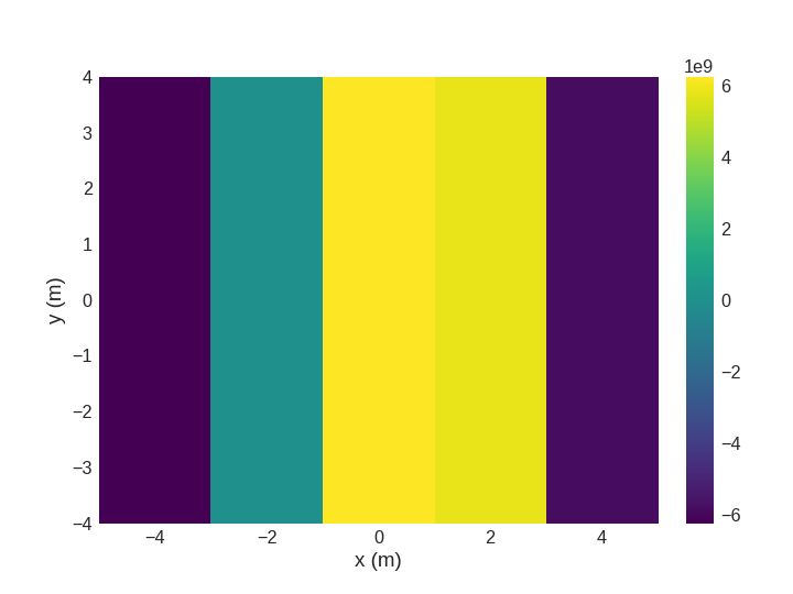
Visualising the phase using
matplotlib.
>>> import discretisedfield as df
>>> import mag2exp
>>> mesh = df.Mesh(p1=(-5, -4, -1), p2=(5, 4, 1), cell=(2, 1, 0.5))
...
>>> def value_fun(point):
...     x, y, z = point
...     if x > 0:
...         return (0, -1, 0)
...     else:
...         return (0, 1, 0)
...
>>> field = df.Field(mesh, nvdim=3, value=value_fun)
>>> phase, ft_phase = mag2exp.ltem.phase(field)
>>> phase.mpl.scalar()