Table visualisation

Table object provides a convenience function which allows us to plot the data stored. Plotting is performed using matplotlib and the method is mpl.

Let us demonstrate plotting using the data from an example file:

import os

import ubermagtable as ut

# Sample OOMMF .odt file
dirname = os.path.join("..", "ubermagtable", "tests", "test_sample")
odtfile = os.path.join(dirname, "oommf-old-file2.odt")

table = ut.Table.fromfile(odtfile, x="t")

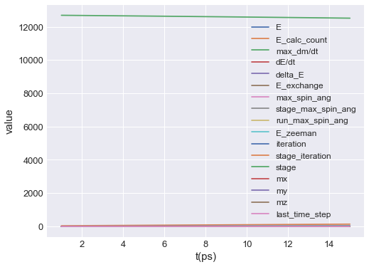
By calling mpl method, default plot is shown:

table.mpl()

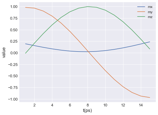
By default, all data columns are plotted. To select only certain data columns, y can be passed. y is a list of strings, where each string matches one of the columns. For instance, if we want to plot the average magnetisation components, the plot is:

table.mpl(y=["mx", "my", "mz"])

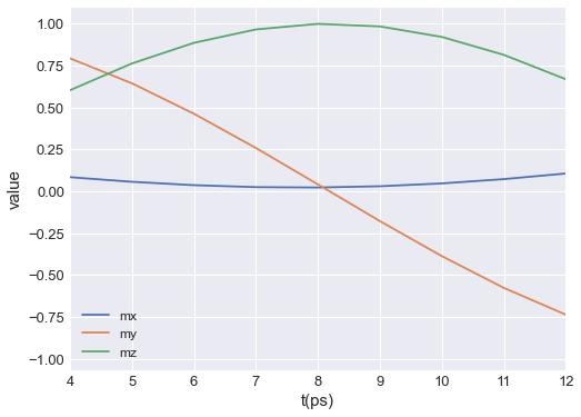
Data columns are always plotted over the entire range of independent variable values. If we want to restrict it, we can pass xlim, which is a lenght-2 tuple defining the range of time values on the horizontal axis:

table.mpl(y=["mx", "my", "mz"], xlim=(4e-12, 12e-12))

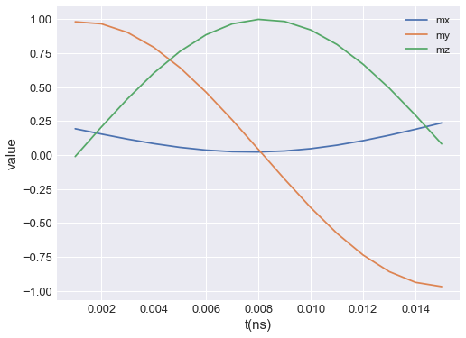
ubermagtable automatically chooses the SI prefix (nano, micro, etc.) it is going to use to divide the horizontal axis with and show those units on the axes. Sometimes ubermagtable does not choose the SI prefix we expected. In those cases, we can explicitly pass it using multiplier argument. multiplier can be passed as \(10^{n}\), where \(n\) is a multiple of 3 (…, -6, -3, 0, 3, 6,…). For instance, if multiplier=1e-9 is passed, all axes will be divided by \(1\,\text{ns}\) and \(\text{ns}\) units will be used as axis labels.

table.mpl(y=["mx", "my", "mz"], multiplier=1e-9)

If we want to save the plot, we pass filename, mesh plot is going to be shown and the plot will be saved in our working directory as a PDF.

table.mpl(y=["mx", "my", "mz"], filename="my-table-plot.pdf")

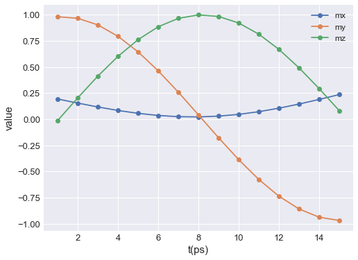
mpl plot is based on `matplotlib.pyplot.plot function <https://matplotlib.org/3.2.1/api/_as_gen/matplotlib.pyplot.plot.html>`__. Therefore, any parameter accepted by it can be passed. For instance:

table.mpl(y=["mx", "my", "mz"], marker="o")

Finally, we show how to expose the axes on which the mesh is plotted, so that we can customise them. We do that by creating the axes ourselves and then passing them to mpl function.

import matplotlib.pyplot as plt

# Create the axes
fig = plt.figure(figsize=(8, 5))
ax = fig.add_subplot(111)

# Add the region to the axes
table.mpl(ax=ax, y=["mx", "my", "mz"])

# Customise the axes
ax.set_xlabel("time in picoseconds")
ax.set_ylabel("average magnetisation")

Text(0, 0.5, 'average magnetisation')

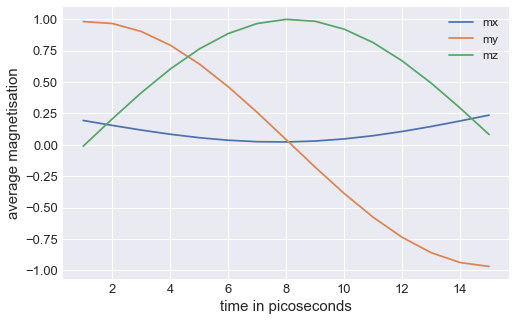
This way, by exposing the axes and passing any allowed matplotlib.pyplot.plot argument, we can customise the plot any way we like (as long as it is allowed by matplotlib).

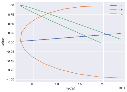
We can also choose what we want as an independent variable on out plot:

table.mpl(x="mx", y=["mx", "my", "mz"])