Field#

class discretisedfield.Field(mesh, nvdim=None, value=0.0, norm=None, vdims=None, dtype=None, unit=None, valid=True, vdim_mapping=None, **kwargs)#

Finite-difference field.

This class specifies a finite-difference field and defines operations for its analysis and visualisation. The field is defined on a finite-difference mesh (discretisedfield.Mesh) passed using mesh. Another value that must be passed is the dimension of the field’s value using nvdim. For instance, for a scalar field, nvdim=1 and for a three-dimensional vector field nvdim=3 must be passed. The value of the field can be set by passing value. For details on how the value can be defined, refer to discretisedfield.Field.value. Similarly, if the field has nvdim>1, the field can be normalised by passing norm. For details on setting the norm, please refer to discretisedfield.Field.norm.

Parameters:

mesh (discretisedfield.Mesh) – Finite-difference rectangular mesh.
nvdim (int) – Number of Value dimensions of the field. For instance, if nvdim=3 the field is a three-dimensional vector field and for nvdim=1 the field is a scalar field.
value (array_like, callable, dict, optional) – Please refer to discretisedfield.Field.value property. Defaults to 0, meaning that if the value is not provided in the initialisation, “zero-field” will be defined.
norm (numbers.Real, callable, optional) – Please refer to discretisedfield.Field.norm property. Defaults to None (norm=None defines no norm).
dtype (str, type, np.dtype, optional) – Data type of the underlying numpy array. If not specified the best data type is automatically determined if value is array_like, for callable and dict value the numpy default (currently float64) is used. Defaults to None.
unit (str, optional) – Physical unit of the field.
valid (numpy.ndarray, str, optional) – Property used to mask invalid values of the field. Please refer to discretisedfield.Field.valid. Defaults to True.
vdim_mapping (dict, optional) – Dictionary that maps value dimensions to the spatial dimensions. It defaults to the same as spatial dimensions if the number of value and spatial dimensions are the same, else it is empty.

Examples

1. Defining a uniform three-dimensional vector field on a nano-sized thin film.

>>> import discretisedfield as df
...
>>> p1 = (-50e-9, -25e-9, 0)
>>> p2 = (50e-9, 25e-9, 5e-9)
>>> cell = (1e-9, 1e-9, 0.1e-9)
>>> mesh = df.Mesh(region=df.Region(p1=p1, p2=p2), cell=cell)
>>> nvdim = 3
>>> value = (0, 0, 1)
...
>>> field = df.Field(mesh=mesh, nvdim=nvdim, value=value)
>>> field
Field(...)
>>> field.mean()
array([0., 0., 1.])

Defining a scalar field.

>>> p1 = (-10, -10, -10)
>>> p2 = (10, 10, 10)
>>> n = (1, 1, 1)
>>> mesh = df.Mesh(p1=p1, p2=p2, n=n)
>>> nvdim = 1
>>> value = 3.14
...
>>> field = df.Field(mesh=mesh, nvdim=nvdim, value=value)
>>> field
Field(...)
>>> field.mean()
array([3.14])

Defining a uniform three-dimensional normalised vector field.

>>> import discretisedfield as df
...
>>> p1 = (-50e9, -25e9, 0)
>>> p2 = (50e9, 25e9, 5e9)
>>> cell = (1e9, 1e9, 0.1e9)
>>> mesh = df.Mesh(region=df.Region(p1=p1, p2=p2), cell=cell)
>>> nvdim = 3
>>> value = (0, 0, 8)
>>> norm = 1
...
>>> field = df.Field(mesh=mesh, nvdim=nvdim, value=value, norm=norm)
>>> field
Field(...)
>>> field.mean()
array([0., 0., 1.])

See also

Mesh()

Methods

`__abs__`	Absolute value of the field.
`__add__`	Binary `+` operator.
`__and__`
`__array_ufunc__`	Field class support for numpy `ufuncs`.
`__call__`	Sample the field value at `point`.
`__dir__`	Extension of the `dir(self)` list.
`__eq__`	Relational operator `==`.
`__getattr__`	Extract the component of the vector field.
`__getitem__`	Extracts the field on a subregion.
`__iter__`	Generator yielding field values of all discretisation cells.
`__lshift__`	Stacks multiple scalar fields in a single vector field.
`__matmul__`
`__mul__`	Binary `*` operator.
`__neg__`	Unary `-` operator.
`__pos__`	Unary `+` operator.
`__pow__`	Unary `**` operator.
`__repr__`	Representation string.
`__sub__`	Binary `-` operator.
`__truediv__`	Binary `/` operator.
`allclose`	Allclose method.
`angle`	Angle between two vectors.
`cross`	Cross product.
`diff`	Directional derivative.
`dot`	Dot product.
`fftn`	Performs an N-dimensional discrete Fast Fourier Transform (FFT) on the field.
`from_file`	Read a field from an OVF (1.0 or 2.0), VTK, or HDF5 file.
`from_xarray`	Create `discretisedfield.Field` from `xarray.DataArray`
`fromfile`
`ifftn`	Performs an N-dimensional discrete inverse Fast Fourier Transform (iFFT) on the field.
`integrate`	Integral.
`irfftn`	Performs an N-dimensional discrete inverse real Fast Fourier Transform (irFFT) on the field.
`is_same_vectorspace`
`line`	Sample the field along the line.
`mean`	Field mean.
`pad`	Field padding.
`resample`	Resample field.
`rfftn`	Performs an N-dimensional discrete real Fast Fourier Transform (rFFT) on the field.
`rotate90`	Rotate field and underlying mesh by 90°.
`sel`	Select a part of the field.
`to_file`	Write the field to OVF, HDF5, or VTK file.
`to_vtk`	Convert field to vtk rectilinear grid.
`to_xarray`	Field value as `xarray.DataArray`.
`update_field_values`	Set field value representation.

Properties

`dtype`
`abs`	Absolute value of complex field.
`array`	Field value as `numpy.ndarray`.
`conjugate`	Complex conjugate of complex field.
`curl`	Curl.
`div`	Compute the divergence of a field.
`grad`	Gradient.
`hv`	Plot interface, Holoviews/hvplot based.
`imag`	Imaginary part of complex field.
`k3d`	Plot interface, k3d based.
`laplace`	Laplace operator.
`mesh`	The mesh on which the field is defined.
`mpl`	Plot interface, matplotlib based.
`norm`	Norm of the field.
`nvdim`	Number of value dimensions.
`orientation`	Orientation field.
`phase`	Phase of complex field.
`real`	Real part of complex field.
`unit`	Unit of the field.
`valid`	Valid field values.
`vdim_mapping`	Map vdims to dims.
`vdims`	Vector components of the field.

__abs__()#

Absolute value of the field.

This is a convenience operator and it returns absolute value of the field.

Returns:: Absolute value of the field.
Return type:: discretisedfield.Field

Examples

Computing the absolute value of a scalar field.

>>> import discretisedfield as df
...
>>> p1 = (0, 0, 0)
>>> p2 = (5, 10, 13)
>>> cell = (1, 1, 1)
>>> mesh = df.Mesh(region=df.Region(p1=p1, p2=p2), cell=cell)
...
>>> field = df.Field(mesh=mesh, nvdim=1, value=-5)
>>> abs(field).mean()
array([5.])

See also

norm()

__add__(other)#

Binary + operator.

It can be applied between two discretisedfield.Field objects or between a discretisedfield.Field object and a “constant”. For instance if the field is a scalar field, a scalar field or numbers.Real can be the second operand. Similarly, for a vector field, either vector field or an iterable, such as tuple, list, or numpy.ndarray, can be the second operand. If the second operand is a discretisedfield.Field object, both must be defined on the same mesh and have the same dimensions.

Parameters:: other (discretisedfield.Field, numbers.Real, tuple, list, np.ndarray) – Second operand.
Returns:: Resulting field.
Return type:: discretisedfield.Field
Raises:: ValueError, TypeError – If the operator cannot be applied.

Example

Add vector fields.

>>> import discretisedfield as df
...
>>> p1 = (0, 0, 0)
>>> p2 = (5, 3, 1)
>>> cell = (1, 1, 1)
>>> mesh = df.Mesh(p1=p1, p2=p2, cell=cell)
...
>>> f1 = df.Field(mesh, nvdim=3, value=(0, -1, -3.1))
>>> f2 = df.Field(mesh, nvdim=3, value=(0, 1, 3.1))
>>> res = f1 + f2
>>> res.mean()
array([0., 0., 0.])
>>> f1 + f2 == f2 + f1
True
>>> res = f1 + (1, 2, 3.1)
>>> res.mean()
array([1., 1., 0.])
>>> (f1 + 5).mean()
array([5. , 4. , 1.9])

See also

__sub__()

__array_ufunc__(ufunc, method, *inputs, **kwargs)#: Field class support for numpy ufuncs.

__call__(point)#

Sample the field value at point.

It returns the value of the field in the discretisation cell to which point belongs to. It returns a tuple, whose length is the same as the dimension (nvdim) of the field.

Parameters:: point (array_like) – For example, in three dimensions, the mesh point coordinate \(\mathbf{p} = (p_{x}, p_{y}, p_{z})\).
Returns:: A tuple, whose length is the same as the dimension of the field.
Return type:: tuple

Example

Sampling the field value.

>>> import discretisedfield as df
...
>>> p1 = (0, 0, 0)
>>> p2 = (20, 20, 20)
>>> n = (20, 20, 20)
>>> mesh = df.Mesh(region=df.Region(p1=p1, p2=p2), n=n)
...
>>> field = df.Field(mesh, nvdim=3, value=(1, 3, 4))
>>> point = (10, 2, 3)
>>> field(point)
array([1., 3., 4.])

__dir__()#

Extension of the dir(self) list.

Adds component labels to the dir(self) list. Similarly, adds or removes methods (grad, div,…) depending on the dimension of the field.

Returns:: Avalilable attributes.
Return type:: list

__eq__(other)#

Relational operator ==.

Two fields are considered to be equal if:

They are defined on the same mesh.

They have the same number of value dimensions (nvdim).

They both contain the same values in array.

Parameters:: other (discretisedfield.Field) – Second operand.
Returns:: True if two fields are equal, False otherwise.
Return type:: bool

Examples

Check if two fields are (not) equal.

>>> import discretisedfield as df
...
>>> mesh = df.Mesh(p1=(0, 0, 0), p2=(5, 5, 5), cell=(1, 1, 1))
...
>>> f1 = df.Field(mesh, nvdim=1, value=3)
>>> f2 = df.Field(mesh, nvdim=1, value=4-1)
>>> f3 = df.Field(mesh, nvdim=3, value=(1, 4, 3))
>>> f1 == f2
True
>>> f1 != f2
False
>>> f1 == f3
False
>>> f1 != f3
True
>>> f2 == f3
False
>>> f1 == 'a'
False

__getattr__(attr)#

Extract the component of the vector field.

This method provides access to individual field components for fields with dimension > 1. Component labels are defined in the vdims attribute. For dimension 2 and 3 default values 'x', 'y', and 'z' are used if no custom component labels are provided. For fields with nvdim>3 vdims must be specified manually to get access to individual vector components.

Parameters:: attr (str) – Vector field component defined in vdims.
Returns:: Scalar field with vector field component values.
Return type:: discretisedfield.Field

Examples

Accessing the default vector field vdims.

>>> import discretisedfield as df
...
>>> p1 = (0, 0, 0)
>>> p2 = (2, 2, 2)
>>> cell = (1, 1, 1)
>>> mesh = df.Mesh(p1=p1, p2=p2, cell=cell)
...
>>> field = df.Field(mesh=mesh, nvdim=3, value=(0, 0, 1))
>>> field.x
Field(...)
>>> field.x.mean()
array([0.])
>>> field.y
Field(...)
>>> field.y.mean()
array([0.])
>>> field.z
Field(...)
>>> field.z.mean()
array([1.])
>>> field.z.nvdim
1

Accessing custom vector field vdims.

>>> import discretisedfield as df
...
>>> p1 = (0, 0, 0)
>>> p2 = (2, 2, 2)
>>> cell = (1, 1, 1)
>>> mesh = df.Mesh(p1=p1, p2=p2, cell=cell)
...
>>> field = df.Field(mesh=mesh, nvdim=3, value=(0, 0, 1),
...                  vdims=['mx', 'my', 'mz'])
>>> field.mx
Field(...)
>>> field.mx.mean()
array([0.])
>>> field.my
Field(...)
>>> field.my.mean()
array([0.])
>>> field.mz
Field(...)
>>> field.mz.mean()
array([1.])
>>> field.mz.nvdim
1

__getitem__(item)#

Extracts the field on a subregion.

If subregions were defined by passing subregions dictionary when the mesh was created, this method returns a field in a subregion subregions[item]. Alternatively, a discretisedfield.Region object can be passed and a minimum-sized field containing it will be returned. The resulting mesh has the same discretisation cell as the original field’s mesh.

Parameters:: item (str, discretisedfield.Region) – The key of a subregion in subregions dictionary or a region object.
Returns:: Field on a subregion.
Return type:: disretisedfield.Field

Example

Extract field on the subregion by passing a key.

>>> import discretisedfield as df
...
>>> p1 = (0, 0, 0)
>>> p2 = (100, 100, 100)
>>> cell = (10, 10, 10)
>>> subregions = {'r1': df.Region(p1=(0, 0, 0), p2=(50, 100, 100)),
...               'r2': df.Region(p1=(50, 0, 0), p2=(100, 100, 100))}
>>> mesh = df.Mesh(p1=p1, p2=p2, cell=cell, subregions=subregions)
>>> def value_fun(point):
...     x, y, z = point
...     if x <= 50:
...         return (1, 2, 3)
...     else:
...         return (-1, -2, -3)
...
>>> f = df.Field(mesh, nvdim=3, value=value_fun)
>>> f.mean()
array([0., 0., 0.])
>>> f['r1']
Field(...)
>>> f['r1'].mean()
array([1., 2., 3.])
>>> f['r2'].mean()
array([-1., -2., -3.])

Extracting a subfield by passing a region.

>>> import discretisedfield as df
...
>>> p1 = (-50e-9, -25e-9, 0)
>>> p2 = (50e-9, 25e-9, 5e-9)
>>> cell = (5e-9, 5e-9, 5e-9)
>>> region = df.Region(p1=p1, p2=p2)
>>> mesh = df.Mesh(region=region, cell=cell)
>>> field = df.Field(mesh=mesh, nvdim=1, value=5)
...
>>> subregion = df.Region(p1=(-9e-9, -1e-9, 1e-9),
...                       p2=(9e-9, 14e-9, 4e-9))
>>> subfield = field[subregion]
>>> subfield.array.shape
(4, 4, 1, 1)

__iter__()#

Generator yielding field values of all discretisation cells.

Yields:: np.ndarray – The field value in one discretisation cell.

Examples

Iterating through the field values

>>> import discretisedfield as df
...
>>> p1 = (0, 0, 0)
>>> p2 = (2, 2, 1)
>>> cell = (1, 1, 1)
>>> mesh = df.Mesh(p1=p1, p2=p2, cell=cell)
...
>>> field = df.Field(mesh, nvdim=3, value=(0, 0, 1))
>>> for value in field:
...     print(value)
[0. 0. 1.]
[0. 0. 1.]
[0. 0. 1.]
[0. 0. 1.]

Iterating through the mesh coordinates and field values

>>> import discretisedfield as df
...
>>> p1 = (0, 0, 0)
>>> p2 = (2, 2, 1)
>>> cell = (1, 1, 1)
>>> mesh = df.Mesh(p1=p1, p2=p2, cell=cell)
...
>>> field = df.Field(mesh, nvdim=3, value=(0, 0, 1))
>>> for coord, value in zip(field.mesh, field):
...     print(coord, value)
[0.5 0.5 0.5] [0. 0. 1.]
[1.5 0.5 0.5] [0. 0. 1.]
[0.5 1.5 0.5] [0. 0. 1.]
[1.5 1.5 0.5] [0. 0. 1.]

See also

__iter__(), indices()

__lshift__(other)#

Stacks multiple scalar fields in a single vector field.

This method takes a list of scalar (nvdim=1) fields and returns a vector field, whose components are defined by the scalar fields passed. If any of the fields passed has nvdim!=1 or they are not defined on the same mesh, an exception is raised. The dimension of the resulting field is equal to the length of the passed list.

Parameters:: fields (list) – List of discretisedfield.Field objects, each with nvdim=1.
Returns:: Resulting field.
Return type:: disrectisedfield.Field
Raises:: ValueError – If the dimension of any of the fields is not 1, or the fields passed are not defined on the same mesh.

Example

Stack 3 scalar fields.

>>> import discretisedfield as df
...
>>> p1 = (0, 0, 0)
>>> p2 = (10, 10, 10)
>>> cell = (2, 2, 2)
>>> mesh = df.Mesh(p1=p1, p2=p2, cell=cell)
...
>>> f1 = df.Field(mesh, nvdim=1, value=1)
>>> f2 = df.Field(mesh, nvdim=1, value=5)
>>> f3 = df.Field(mesh, nvdim=1, value=-3)
...
>>> f = f1 << f2 << f3
>>> f.mean()
array([ 1.,  5., -3.])
>>> f.nvdim
3
>>> f.x == f1
True
>>> f.y == f2
True
>>> f.z == f3
True

__mul__(other)#

Binary * operator.

It can be applied between:

Two fields with equal vector dimensions nvdim,
A field of any dimension nvdim and numbers.Complex,
A field of any dimension nvdim and a scalar (nvdim=1) field.

If both operands are discretisedfield.Field objects, they must be defined on the same mesh.

Parameters:: other (discretisedfield.Field, numbers.Real) – Second operand.
Returns:: Resulting field.
Return type:: discretisedfield.Field
Raises:: ValueError, TypeError – If the operator cannot be applied.

Example

Multiply two scalar fields.

>>> import discretisedfield as df
...
>>> p1 = (0, 0, 0)
>>> p2 = (10, 10, 10)
>>> cell = (2, 2, 2)
>>> mesh = df.Mesh(p1=p1, p2=p2, cell=cell)
...
>>> f1 = df.Field(mesh, nvdim=1, value=5)
>>> f2 = df.Field(mesh, nvdim=1, value=9)
>>> res = f1 * f2
>>> res.mean()
array([45.])
>>> f1 * f2 == f2 * f1
True

Multiply vector field with a scalar.

>>> f1 = df.Field(mesh, nvdim=3, value=(0, 2, 5))
...
>>> res = f1 * 5  # discretisedfield.Field.__mul__ is called
>>> res.mean()
array([ 0., 10., 25.])
>>> res = 10 * f1  # discretisedfield.Field.__rmul__ is called
>>> res.mean()
array([ 0., 20., 50.])

See also

__truediv__()

__neg__()#

Unary - operator.

This method negates the value of each discretisation cell. It is equivalent to multiplication with -1:

\[-f(x, y, z) = -1 \cdot f(x, y, z)\]

Returns:: Field multiplied with -1.
Return type:: discretisedfield.Field

Example

Applying unary - operator on a scalar field.

>>> import discretisedfield as df
...
>>> p1 = (0, 0, 0)
>>> p2 = (5e-9, 3e-9, 1e-9)
>>> n = (10, 5, 1)
>>> mesh = df.Mesh(p1=p1, p2=p2, n=n)
...
>>> f = df.Field(mesh, nvdim=1, value=3.1)
>>> res = -f
>>> res.mean()
array([-3.1])
>>> f == -(-f)
True

Applying unary negation operator on a vector field.

>>> f = df.Field(mesh, nvdim=3, value=(0, -1000, -3))
>>> res = -f
>>> res.mean()
array([   0., 1000.,    3.])

__pos__()#

Unary + operator.

This method defines the unary operator +. It returns the field itself:

\[+f(x, y, z) = f(x, y, z)\]

Returns:: Field itself.
Return type:: discretisedfield.Field

Example

Applying unary + operator on a field.

>>> import discretisedfield as df
...
>>> p1 = (0, 0, 0)
>>> p2 = (5e-9, 5e-9, 5e-9)
>>> n = (10, 10, 10)
>>> mesh = df.Mesh(p1=p1, p2=p2, n=n)
...
>>> f = df.Field(mesh, nvdim=3, value=(0, -1000, -3))
>>> res = +f
>>> res.mean()
array([    0., -1000.,    -3.])
>>> res == f
True
>>> +(+f) == f
True

__pow__(other)#

Unary ** operator.

This method defines the ** operator for scalar (nvdim=1) fields only. This operator is not defined for vector (nvdim>1) fields, and ValueError is raised.

Parameters:: other (numbers.Real) – Value to which the field is raised.
Returns:: Resulting field.
Return type:: discretisedfield.Field
Raises:: ValueError, TypeError – If the operator cannot be applied.

Example

Applying unary ** operator on a scalar field.

>>> import discretisedfield as df
...
>>> p1 = (-25e-3, -25e-3, -25e-3)
>>> p2 = (25e-3, 25e-3, 25e-3)
>>> n = (10, 10, 10)
>>> mesh = df.Mesh(region=df.Region(p1=p1, p2=p2), n=n)
...
>>> f = df.Field(mesh, nvdim=1, value=2)
>>> res = f**(-1)
>>> res
Field(...)
>>> res.mean()
array([0.5])
>>> res = f**2
>>> res.mean()
array([4.])
>>> (f**f).mean()
array([4.])

Attempt to apply power operator on a vector field.

>>> p1 = (0, 0, 0)
>>> p2 = (5e-9, 5e-9, 5e-9)
>>> n = (10, 10, 10)
>>> mesh = df.Mesh(p1=p1, p2=p2, n=n)
...
>>> f = df.Field(mesh, nvdim=3, value=(0, -1, -3))
>>> (f**2).mean()
array([0., 1., 9.])

__repr__()#

Representation string.

Internally self._repr_html_() is called and all html tags are removed from this string.

Returns:: Representation string.
Return type:: str

Example

Getting representation string.

>>> import discretisedfield as df
...
>>> p1 = (0, 0, 0)
>>> p2 = (2, 2, 1)
>>> cell = (1, 1, 1)
>>> mesh = df.Mesh(p1=p1, p2=p2, cell=cell)
...
>>> field = df.Field(mesh, nvdim=1, value=1)
>>> field
Field(...)

__sub__(other)#

Binary - operator.

Parameters:: other (discretisedfield.Field, numbers.Real, tuple, list, np.ndarray) – Second operand.
Returns:: Resulting field.
Return type:: discretisedfield.Field
Raises:: ValueError, TypeError – If the operator cannot be applied.

Example

Subtract vector fields.

>>> import discretisedfield as df
...
>>> p1 = (0, 0, 0)
>>> p2 = (5, 3, 1)
>>> cell = (1, 1, 1)
>>> mesh = df.Mesh(p1=p1, p2=p2, cell=cell)
...
>>> f1 = df.Field(mesh, nvdim=3, value=(0, 1, 6))
>>> f2 = df.Field(mesh, nvdim=3, value=(0, 1, 3))
>>> res = f1 - f2
>>> res.mean()
array([0., 0., 3.])
>>> f1 - f2 == -(f2 - f1)
True
>>> res = f1 - (0, 1, 0)
>>> res.mean()
array([0., 0., 6.])

See also

__add__()

__truediv__(other)#

Binary / operator.

It can be applied between:

Two fields with equal vector dimensions nvdim,
A field of any dimension nvdim and numbers.Complex,
A field of any dimension nvdim and a scalar (nvdim=1) field.

If both operands are discretisedfield.Field objects, they must be defined on the same mesh.

Parameters:: other (discretisedfield.Field, numbers.Real) – Second operand.
Returns:: Resulting field.
Return type:: discretisedfield.Field
Raises:: ValueError, TypeError – If the operator cannot be applied.

Example

Divide two scalar fields.

>>> import discretisedfield as df
...
>>> p1 = (0, 0, 0)
>>> p2 = (10, 10, 10)
>>> cell = (2, 2, 2)
>>> mesh = df.Mesh(p1=p1, p2=p2, cell=cell)
...
>>> f1 = df.Field(mesh, nvdim=1, value=100)
>>> f2 = df.Field(mesh, nvdim=1, value=20)
>>> res = f1 / f2
>>> res.mean()
array([5.])
>>> (f1 / f2).allclose((f2 / f1)**(-1))
True

Divide vector field by a scalar.

>>> f1 = df.Field(mesh, nvdim=3, value=(0, 10, 5))
>>> res = f1 / 5  # discretisedfield.Field.__mul__ is called
>>> res.mean()
array([0., 2., 1.])
>>> (10 / f1).mean()  # division by a vector is not allowed
array([inf,  1.,  2.])

See also

__mul__()

allclose(other, rtol=1e-05, atol=1e-08)#

Allclose method.

This method determines whether two fields are:

Defined on the same mesh.

Have the same number of value dimension (nvdim).

3. All values in are within relative (rtol) and absolute (atol) tolerances.

Parameters:

other (discretisedfield.Field) – Field to be compared to.
rtol (numbers.Real) – Relative tolerance. Defaults to 1e-5.
atol (numbers.Real) – Absolute tolerance. Defaults to 1e-8.

Returns:

True if two fields are within tolerance, False otherwise.

Return type:

bool

Raises:

TypeError – If a non field object is passed.

Examples

Check if two fields are within a tolerance.

>>> import discretisedfield as df
...
>>> mesh = df.Mesh(p1=(0, 0, 0), p2=(5, 5, 5), cell=(1, 1, 1))
...
>>> f1 = df.Field(mesh, nvdim=1, value=3)
>>> f2 = df.Field(mesh, nvdim=1, value=3+1e-9)
>>> f3 = df.Field(mesh, nvdim=1, value=3.1)
>>> f1.allclose(f2)
True
>>> f1.allclose(f3)
False
>>> f1.allclose(f3, atol=1e-2)
False

angle(vector)#

Angle between two vectors.

It can be applied between two discretisedfield.Field objects. For a vector field, the second operand can be a vector in the form of an iterable, such as tuple, list, or numpy.ndarray. If the second operand is a discretisedfield.Field object, both must be defined on the same mesh and have the same dimensions. This method then returns a scalar field which is an angle between the component of the vector field and a vector. The angle is computed in radians and all values are in \((0, 2\pi)\) range.

Parameters:: other (discretisedfield.Field, numbers.Real, tuple, list, np.ndarray) – Second operand.
Returns:: Angle scalar field.
Return type:: discretisedfield.Field
Raises:: ValueError, TypeError – If the field is not sliced.

Example

Computing the angle of the field in yz-plane.

>>> import discretisedfield as df
>>> import numpy as np
...
>>> p1 = (0, 0, 0)
>>> p2 = (100, 100, 100)
>>> n = (10, 10, 10)
>>> mesh = df.Mesh(p1=p1, p2=p2, n=n)
>>> field = df.Field(mesh, nvdim=3, value=(0, 1, 0))
...
>>> field.angle((1, 0, 0)).mean()
array([1.57079633])

cross(other)#

Cross product.

This method computes the cross product between two fields. Both fields must be three-dimensional (nvdim=3) and defined on the same mesh.

Parameters:: other (discretisedfield.Field, tuple, list, numpy.ndarray) – Second operand.
Returns:: Resulting field.
Return type:: discretisedfield.Field
Raises:: ValueError, TypeError – If the operator cannot be applied.

Example

Compute the cross product of two vector fields.

>>> import discretisedfield as df
...
>>> p1 = (0, 0, 0)
>>> p2 = (10, 10, 10)
>>> cell = (2, 2, 2)
>>> mesh = df.Mesh(p1=p1, p2=p2, cell=cell)
...
>>> f1 = df.Field(mesh, nvdim=3, value=(1, 0, 0))
>>> f2 = df.Field(mesh, nvdim=3, value=(0, 1, 0))
>>> (f1.cross(f2)).mean()
array([0., 0., 1.])
>>> (f1.cross((0, 0, 1))).mean()
array([ 0., -1.,  0.])

diff(direction, order=1, restrict2valid=True)#

Directional derivative.

This method computes a directional derivative of the field and returns a field. The direction in which the derivative is computed is passed via direction argument, which can be any element of region.dims. The order of the computed derivative can be 1 or 2 and it is specified using argument order and it defaults to 1.

This method uses second order accurate finite difference stencils by default unless the field is defined on a mesh with too few cells in the differential direction. In this case the first order accurate finite difference stencils are used at the boundaries and the second order accurate finite difference stencils are used in the interior.

Directional derivative cannot be computed if less or equal discretisation cells exists in a specified direction than the order. In that case, a zero field is returned.

By default, the directional derivative is computed only across contiguous areas of the field where the field is valid. This behaviour can be changed to compute the directional derivative across the whole field by setting restrict2valid to False.

Computing of the directional derivative depends strongly on the boundary condition specified. In this method, only periodic boundary conditions at the edges of the region are supported. To enable periodic boundary conditions, set mesh.bc.

Parameters:

direction (str) – The spatial direction in which the derivative is computed.
order (int) – The order of the derivative. It can be 1 or 2 and it defaults to 1.
restrict2valid (bool) – If True, the directional derivative is computed only across contiguous areas of the field where the field is valid. If False, the directional derivative is computed across the whole field. The default value is True.

Returns:

Directional derivative.

Return type:

discretisedfield.Field

Raises:

NotImplementedError – If order n higher than 2 is asked for.

Example

1. Compute the first-order directional derivative of a scalar field in the y-direction of a spatially varying field. For the field we choose \(f(x, y, z) = 2x + 3y - 5z\). Accordingly, we expect the derivative in the y-direction to be to be a constant scalar field \(df/dy = 3\).

>>> import discretisedfield as df
...
>>> p1 = (0, 0, 0)
>>> p2 = (100e-9, 100e-9, 10e-9)
>>> cell = (10e-9, 10e-9, 10e-9)
>>> mesh = df.Mesh(p1=p1, p2=p2, cell=cell)
...
>>> def value_fun(point):
...     x, y, z = point
...     return 2*x + 3*y + -5*z
...
>>> f = df.Field(mesh, nvdim=1, value=value_fun)
>>> f.diff('y').mean()  # first-order derivative by default
array([3.])

2. Try to compute the second-order directional derivative of the vector field which has only one discretisation cell in the z-direction. For the field we choose \(f(x, y, z) = (2x, 3y, -5z)\). Accordingly, we expect the directional derivatives to be: \(df/dx = (2, 0, 0)\), \(df/dy=(0, 3, 0)\), \(df/dz = (0, 0, -5)\). However, because there is only one discretisation cell in the z-direction, the derivative cannot be computed and a zero field is returned.

>>> import numpy as np
>>> def value_fun(point):
...     x, y, z = point
...     return (2*x, 3*y, -5*z)
...
>>> f = df.Field(mesh, nvdim=3, value=value_fun)
>>> np.allclose(f.diff('x', order=1).mean(), [2, 0, 0])
True
>>> np.allclose(f.diff('y', order=1).mean(), [0, 3, 0])
True
>>> f.diff('z', order=1).mean()  # derivative cannot be calculated
array([0., 0., 0.])

3. Compute the second-order directional derivative of a scalar field with which is only valid below x=5.

>>> def value_fun(point):
...     x = point
...     return x
...
>>> def valid_fun(point):
...     x = point
...     return x < 5
...
>>> mesh = df.Mesh(p1=0, p2=10, cell=1)
>>> f = df.Field(mesh, nvdim=1, value=value_fun, valid=valid_fun)
>>> f.diff('x', order=1).array.tolist()
[[1.0], [1.0], [1.0], [1.0], [1.0], [0.0], [0.0], [0.0], [0.0], [0.0]]

dot(other)#

Dot product.

This method computes the dot product between two fields. Both fields must have the same number of vector dimentions and defined on the same mesh

Parameters:: other (discretisedfield.Field) – Second operand.
Returns:: Resulting field.
Return type:: discretisedfield.Field
Raises:: ValueError, TypeError – If the operator cannot be applied.

Example

Compute the dot product of two vector fields.

>>> import discretisedfield as df
...
>>> p1 = (0, 0, 0)
>>> p2 = (10e-9, 10e-9, 10e-9)
>>> cell = (2e-9, 2e-9, 2e-9)
>>> mesh = df.Mesh(p1=p1, p2=p2, cell=cell)
...
>>> f1 = df.Field(mesh, nvdim=3, value=(1, 3, 6))
>>> f2 = df.Field(mesh, nvdim=3, value=(-1, -2, 2))
>>> f1.dot(f2).mean()
array([5.])

fftn(**kwargs)#

Performs an N-dimensional discrete Fast Fourier Transform (FFT) on the field.

This method applies an FFT to the field and the underying mesh, transforming it from a spatial domain into a frequency domain. During this process, any information about subregions within the field is lost.

Parameters:: **kwargs – Keyword arguments passed directly to the FFT function provided by SciPy’s fftpack scipy.fft.fftn().
Returns:: A field representing the Fourier transform of the original field. This returned field has value dimensions labeled with frequency (ft_ in front of each vdim) and values corresponding to frequencies in the frequency domain.
Return type:: discretisedfield.Field

Examples

1. Create a mesh and perform an FFT. >>> import discretisedfield as df >>> mesh = df.Mesh(p1=0, p2=10, cell=2) >>> field = df.Field(mesh, nvdim=3, value=(1, 2, 3)) >>> fft_field = field.fftn() >>> fft_field.nvdim 3 >>> fft_field.vdims [‘ft_x’, ‘ft_y’, ‘ft_z’]

2. Create a 3D mesh and perform an FFT. >>> import discretisedfield as df >>> mesh = df.Mesh(p1=(0, 0, 0), p2=(10, 10, 10), cell=(2, 2, 2)) >>> field = df.Field(mesh, nvdim=4, value=(1, 2, 3, 4)) >>> fft_field = field.fftn() >>> fft_field.nvdim 4 >>> fft_field.vdims [‘ft_v0’, ‘ft_v1’, ‘ft_v2’, ‘ft_v3’]

classmethod from_xarray(xa)#

Create discretisedfield.Field from xarray.DataArray

The class method accepts an xarray.DataArray as an argument to return a discretisedfield.Field object. The first n (or n-1) dimensions of the DataArray are considered geometric dimensions of a scalar (or vector) field. In case of a vector field, the last dimension must be named vdims. The DataArray attribute nvdim determines whether it is a scalar or a vector field (i.e. nvdim = 1 is a scalar field and nvdim >= 1 is a vector field). Hence, nvdim attribute must be present, greater than or equal to one, and of an integer type.

The DataArray coordinates corresponding to the geometric dimensions represent the discretisation along the respective dimension and must have equally spaced values. The coordinates of vdims represent the name of field components (e.g. [‘x’, ‘y’, ‘z’] for a 3D vector field).

Additionally, it is expected to have cell, p1, and p2 attributes for creating the right mesh for the field; however, in the absence of these, the coordinates of the geometric axes dimensions are utilized. It should be noted that cell attribute is required if any of the geometric directions has only a single cell.

Parameters:

xa (xarray.DataArray) – DataArray to create Field.

Returns:

Field created from DataArray.

Return type:

discretisedfield.Field

Raises:

TypeError –
- If argument is not xarray.DataArray. - If nvdim attribute in not an integer.
KeyError –
- If at least one of the geometric dimension coordinates has a single value and cell attribute is missing. - If nvdim attribute is absent.
ValueError –
- If DataArray does not have a dimension vdims when attribute nvdim is grater than one. - If coordinates of geometrical dimensions are not equally spaced.

Examples

Create a DataArray

>>> import xarray as xr
>>> import numpy as np
...
>>> xa = xr.DataArray(np.ones((20, 20, 20, 3), dtype=float),
...                   dims = ['x', 'y', 'z', 'vdims'],
...                   coords = dict(x=np.arange(0, 20),
...                                 y=np.arange(0, 20),
...                                 z=np.arange(0, 20),
...                                 vdims=['x', 'y', 'z']),
...                   name = 'mag',
...                   attrs = dict(cell=[1., 1., 1.],
...                                p1=[1., 1., 1.],
...                                p2=[21., 21., 21.],
...                                nvdim=3),)
>>> xa
<xarray.DataArray 'mag' (x: 20, y: 20, z: 20, vdims: 3)>
...

Create Field from DataArray

>>> import discretisedfield as df
...
>>> field = df.Field.from_xarray(xa)
>>> field
Field(...)
>>> field.mean()
array([1., 1., 1.])

ifftn(**kwargs)#

Performs an N-dimensional discrete inverse Fast Fourier Transform (iFFT) on the field.

This method applies an iFFT to the field and the underying mesh, transforming it from a frequency domain into a spatial domain. During this process, any information about subregions within the field is lost.

Parameters:: **kwargs – Keyword arguments passed directly to the iFFT function provided by SciPy’s fftpack scipy.fft.ifftn().
Returns:: A field representing the inverse Fourier transform of the original field. This returned field is in the spatial domain and has value dimensions labeled with the ft_ removed if the vdims of the original field started with ft_.
Return type:: discretisedfield.Field

Examples

1. Create a mesh and perform an iFFT. >>> import discretisedfield as df >>> mesh = df.Mesh(p1=0, p2=10, cell=2) >>> field = df.Field(mesh, nvdim=3, value=(1, 2, 3)) >>> ifft_field = field.fftn().ifftn() >>> ifft_field.nvdim 3 >>> ifft_field.vdims [‘x’, ‘y’, ‘z’]

2. Create a 3D mesh and perform an iFFT. >>> import discretisedfield as df >>> mesh = df.Mesh(p1=(0, 0, 0), p2=(10, 10, 10), cell=(2, 2, 2)) >>> field = df.Field(mesh, nvdim=4, value=(1, 2, 3, 4)) >>> fft_field = field.fftn().ifftn() >>> fft_field.nvdim 4 >>> fft_field.vdims [‘v0’, ‘v1’, ‘v2’, ‘v3’]

integrate(direction=None, cumulative=False)#

Integral.

This method integrates the field over the mesh along the specified direction, which can be specified using direction. The field is internally multiplied with the cell size in that direction. If no direction is specified the integral is computed along all directions.

To compute surface integrals, e.g. flux, the field must be multiplied with the surface normal vector prior to integration (see example 4).

A cumulative integral can be computed by passing cumulative=True and by specifying a single direction. It resembles the following integral (here as an example in the x direction):

\[F(x, y, z) = \int_{p_\mathrm{min}}^x f(x', y, z) \mathrm{d}x\]

The method sums all cells up to (excluding) the cell that contains the point x. The cell containing x is added with a weight 1/2.

Parameters:

direction (str, optional) – Direction along which the field is integrated. The direction must be in field.mesh.region.dims. Defaults to None.
cumulative (bool, optional) – If True, an cumulative integral is computed. Defaults to False.

Returns:

Integration result. If the field is integrated in all directions, an np.ndarray is returned.

Return type:

discretisedfield.Field or np.ndarray

Raises:

ValueError – If cumulative=True and no integration direction is specified.

Example

Volume integral of a scalar field.

\[\int_\mathrm{V} f(\mathbf{r}) \mathrm{d}V\]

>>> import discretisedfield as df
...
>>> p1 = (0, 0, 0)
>>> p2 = (10, 10, 10)
>>> cell = (2, 2, 2)
>>> mesh = df.Mesh(p1=p1, p2=p2, cell=cell)
...
>>> f = df.Field(mesh, nvdim=1, value=5)
>>> f.integrate()
array([5000.])

Volume integral of a vector field.

\[\int_\mathrm{V} \mathbf{f}(\mathbf{r}) \mathrm{d}V\]

>>> f = df.Field(mesh, nvdim=3, value=(-1, -2, -3))
>>> f.integrate()
array([-1000., -2000., -3000.])

Surface integral of a scalar field.

\[\int_\mathrm{S} f(\mathbf{r}) |\mathrm{d}\mathbf{S}|\]

>>> f = df.Field(mesh, nvdim=1, value=5)
>>> f_plane = f.sel('z')
>>> f_plane.integrate()
array([500.])

4. Surface integral of a vector field (flux). The dot product with the surface normal vector must be calculated manually.

\[\int_\mathrm{S} \mathbf{f}(\mathbf{r}) \cdot \mathrm{d}\mathbf{S}\]

>>> f = df.Field(mesh, nvdim=3, value=(1, 2, 3))
>>> f_plane = f.sel('z')
>>> e_z = [0, 0, 1]
>>> f_plane.dot(e_z).integrate()
array([300.])

Integral along x-direction.

\[\int_{x_\mathrm{min}}^{x_\mathrm{max}} \mathbf{f}(\mathbf{r}) \mathrm{d}x\]

>>> f = df.Field(mesh, nvdim=3, value=(1, 2, 3))
>>> f_plane = f.sel('z')
>>> f_plane.integrate(direction='x').mean()
array([10., 20., 30.])

Cumulative integral along x-direction.

\[\int_{x_\mathrm{min}}^{x} \mathbf{f}(\mathbf{r}) \mathrm{d}x'\]

>>> f = df.Field(mesh, nvdim=3, value=(1, 2, 3))
>>> f_plane = f.sel('z')
>>> f_plane.integrate(direction='x', cumulative=True)
Field(...)

irfftn(shape=None, **kwargs)#

Performs an N-dimensional discrete inverse real Fast Fourier Transform (irFFT) on the field.

This method applies an irFFT to the field and the underying mesh, transforming it from a frequency domain into a spatial domain. During this process, any information about subregions within the field is lost.

Parameters:: **kwargs – Keyword arguments passed directly to the irFFT function provided by SciPy’s fftpack scipy.fft.irfftn().
Returns:: A field representing the inverse Fourier transform of the original field. This returned field is in the spatial domain and has value dimensions labeled with the ft_ removed if the vdims of the original field started with ft_.
Return type:: discretisedfield.Field

Examples

1. Create a mesh and perform an irFFT. >>> import discretisedfield as df >>> mesh = df.Mesh(p1=0, p2=10, cell=2) >>> field = df.Field(mesh, nvdim=3, value=(1, 2, 3)) >>> ifft_field = field.fftn().irfftn() >>> ifft_field.nvdim 3 >>> ifft_field.vdims [‘x’, ‘y’, ‘z’]

2. Create a 3D mesh and perform an irFFT. >>> import discretisedfield as df >>> mesh = df.Mesh(p1=(0, 0, 0), p2=(10, 10, 10), cell=(2, 2, 2)) >>> field = df.Field(mesh, nvdim=4, value=(1, 2, 3, 4)) >>> fft_field = field.fftn().irfftn() >>> fft_field.nvdim 4 >>> fft_field.vdims [‘v0’, ‘v1’, ‘v2’, ‘v3’]

line(p1, p2, n=100)#

Sample the field along the line.

Given two points \(p_{1}\) and \(p_{2}\), \(n\) position coordinates are generated and the corresponding field values.

\[\mathbf{r}_{i} = i\frac{\mathbf{p}_{2} - \mathbf{p}_{1}}{n-1}\]

Parameters:

p1 (array_like) – Two points between which the line is generated.
p2 (array_like) – Two points between which the line is generated.
n (int, optional) – Number of points on the line. Defaults to 100.

Returns:

Line object.

Return type:

discretisedfield.Line

Raises:

ValueError – If p1 or p2 is outside the mesh domain.

Examples

Sampling the field along the line.

>>> import discretisedfield as df
...
>>> p1 = (0, 0, 0)
>>> p2 = (2, 2, 2)
>>> cell = (1, 1, 1)
>>> mesh = df.Mesh(p1=p1, p2=p2, cell=cell)
>>> field = df.Field(mesh, nvdim=2, value=(0, 3))
...
>>> line = field.line(p1=(0, 0, 0), p2=(2, 0, 0), n=5)

mean(direction=None)#

Field mean.

It computes the arithmetic mean along the specified direction of the field.

It returns a numpy array containing the mean value if all the geometrical directions or none are selected. If one or more than one directions (and less than region.dims) are selected, the method returns a field of appropriate geometric dimensions with the calculated mean value.

Parameters:

direction (None, string or tuple of strings, optional.) – Directions along which the mean is computed. The default is to compute the mean of the entire volume and return an array of the averaged vector components.

Returns:

numpy.ndarray – Field average along all the geometrical directions combined.
discretisedfield.Field – Field of reduced geometrical dimensions holding the mean value along the selected direction(s).

Examples

Computing the vector field average.

>>> import discretisedfield as df
...
>>> p1 = (0, 0, 0)
>>> p2 = (5, 5, 5)
>>> cell = (1, 1, 1)
>>> mesh = df.Mesh(p1=p1, p2=p2, cell=cell)
...
>>> field = df.Field(mesh=mesh, nvdim=3, value=(0, 0, 1))
>>> field.mean()
array([0., 0., 1.])

Computing the scalar field average.

>>> field = df.Field(mesh=mesh, nvdim=1, value=55)
>>> field.mean()
array([55.])

Computing the vector field mean along x direction.

>>> import discretisedfield as df
...
>>> p1 = (0, 0, 0)
>>> p2 = (5, 5, 5)
>>> cell = (1, 1, 1)
>>> mesh = df.Mesh(p1=p1, p2=p2, cell=cell)
...
>>> field = df.Field(mesh=mesh, nvdim=3, value=(0, 0, 1))
>>> field.mean(direction='x')((0.5, 0.5))
array([0., 0., 1.])

Computing the vector field mean along x and y directions.

>>> import discretisedfield as df
...
>>> p1 = (0, 0, 0)
>>> p2 = (5, 5, 5)
>>> cell = (1, 1, 1)
>>> mesh = df.Mesh(p1=p1, p2=p2, cell=cell)
...
>>> field = df.Field(mesh=mesh, nvdim=3, value=(0, 0, 1))
>>> field.mean(direction=['x', 'y'])(0.5)
array([0., 0., 1.])

pad(pad_width, mode, **kwargs)#

Field padding.

This method pads the field by adding more cells in chosen direction and assigning to them the values as specified by the mode argument. The way in which the field is going to padded is defined by passing pad_width dictionary. The keys of the dictionary are the directions (axes), e.g. 'x', 'y', or 'z', whereas the values are the tuples of length 2. The first integer in the tuple is the number of cells added in the negative direction, and the second integer is the number of cells added in the positive direction.

This method accepts any other arguments allowed by numpy.pad function.

Parameters:

pad_width (dict) – The keys of the dictionary are the directions (axes), e.g. 'x', 'y', or 'z', whereas the values are the tuples of length 2. The first integer in the tuple is the number of cells added in the negative direction, and the second integer is the number of cells added in the positive direction.
mode (str) – Padding mode as defined in numpy.pad.

Returns:

Padded field.

Return type:

discretisedfield.Field

Examples

Padding a field in the x direction by 1 cell with constant mode.

>>> import discretisedfield as df
...
>>> p1 = (0, 0, 0)
>>> p2 = (2, 1, 1)
>>> cell = (1, 1, 1)
>>> mesh = df.Mesh(p1=p1, p2=p2, cell=cell)
>>> field = df.Field(mesh, nvdim=1, value=1)
...
>>> # Two cells with value 1
>>> pf = field.pad({'x': (1, 1)}, mode='constant')  # zeros padded
>>> pf.mean()
array([0.5])

resample(n)#

Resample field.

This method computes the field on a new mesh with n cells. The boundaries pmin and pmax stay unchanged. The values of the new cells are taken from the nearest old cell, no interpolation is performed.

Parameters:: n (array_like) – Number of cells in each direction. The number of elements must match field.mesh.region.ndim.
Returns:: The resampled field.
Return type:: discretisedfield.Field

Examples

Decrease the number of cells.

>>> import discretisedfield as df
...
>>> p1 = (0, 0, 0)
>>> p2 = (100, 100, 100)
>>> cell = (10, 10, 10)
>>> mesh = df.Mesh(p1=p1, p2=p2, cell=cell)
>>> f = df.Field(mesh, nvdim=1, value=1)
>>> f.mesh.n
array([10, 10, 10])
>>> down_sampled = f.resample((5, 5, 5))
>>> down_sampled.mesh.n
array([5, 5, 5])

Increase the number of cells.

>>> import discretisedfield as df
...
>>> p1 = (0, 0, 0)
>>> p2 = (100, 100, 100)
>>> cell = (10, 10, 10)
>>> mesh = df.Mesh(p1=p1, p2=p2, cell=cell)
>>> f = df.Field(mesh, nvdim=1, value=1)
>>> f.mesh.n
array([10, 10, 10])
>>> up_sampled = f.resample((10, 15, 20))
>>> up_sampled.mesh.n
array([10, 15, 20])

rfftn(**kwargs)#

Performs an N-dimensional discrete real Fast Fourier Transform (rFFT) on the field.

This method applies an rFFT to the field and the underying mesh, transforming it from a spatial domain into a frequency domain. During this process, any information about subregions within the field is lost.

Parameters:: **kwargs – Keyword arguments passed directly to the rFFT function provided by SciPy’s fftpack scipy.fft.rfftn().
Returns:: A field representing the Fourier transform of the original field. This returned field has value dimensions labeled with frequency (ft_ in front of each vdim) and values corresponding to frequencies in the frequency domain.
Return type:: discretisedfield.Field

Examples

1. Create a mesh and perform an rFFT. >>> import discretisedfield as df >>> mesh = df.Mesh(p1=0, p2=10, cell=2) >>> field = df.Field(mesh, nvdim=3, value=(1, 2, 3)) >>> fft_field = field.rfftn() >>> fft_field.nvdim 3 >>> fft_field.vdims [‘ft_x’, ‘ft_y’, ‘ft_z’]

2. Create a 3D mesh and perform an rFFT. >>> import discretisedfield as df >>> mesh = df.Mesh(p1=(0, 0, 0), p2=(10, 10, 10), cell=(2, 2, 2)) >>> field = df.Field(mesh, nvdim=4, value=(1, 2, 3, 4)) >>> fft_field = field.rfftn() >>> fft_field.nvdim 4 >>> fft_field.vdims [‘ft_v0’, ‘ft_v1’, ‘ft_v2’, ‘ft_v3’]

rotate90(ax1, ax2, k=1, reference_point=None, inplace=False)#

Rotate field and underlying mesh by 90°.

Rotate the field k times by 90 degrees in the plane defined by ax1 and ax2. The rotation direction is from ax1 to ax2, the two must be different.

For vector fields (nvdim>1) the components of the vector pointing along ax1 and ax2 are determined from vdim_mapping. Rotation is only possible if this mapping defines vector components along both directions ax1 and ax2.

Parameters:

ax1 (str) – Name of the first dimension.
ax2 (str) – Name of the second dimension.
k (int, optional) – Number of 90° rotations, defaults to 1.
reference_point (array_like, optional) – Point around which the mesh is rotated. If not provided the mesh.region’s centre point of the field is used.
inplace (bool, optional) – If True, the rotation is applied in-place. Defaults to False.

Returns:

The rotated field object. Either a new object or a reference to the existing field for inplace=True.

Return type:

discretisedfield.Field

Raises:

RuntimeError – If a vector field (nvdim>1) does not provide the required mapping between spatial directions and vector components in vdim_mapping.

Examples

>>> import discretisedfield as df
>>> import numpy as np
>>> p1 = (0, 0, 0)
>>> p2 = (10, 8, 6)
>>> mesh = df.Mesh(p1=p1, p2=p2, n=(10, 4, 6))
>>> field = df.Field(mesh, nvdim=3, value=(1, 2, 3))
>>> rotated = field.rotate90('x', 'y')
>>> rotated.mesh.region.pmin
array([ 1., -1.,  0.])
>>> rotated.mesh.region.pmax
array([9., 9., 6.])
>>> rotated.mesh.n
array([ 4, 10,  6])
>>> rotated.mean()
array([-2.,  1.,  3.])

See also

rotate90(), rotate90()

sel(*args, **kwargs)#

Select a part of the field.

If one of the axis from region.dims is passed as a string, a field of a reduced dimension along the axis and perpendicular to it is extracted, intersecting the axis at its center. Alternatively, if a keyword (representing the axis) argument is passed with a real number value (e.g. x=1e-9), a field of reduced dimensions intersects the axis at a point ‘nearest’ to the provided value is returned. If the mesh is already 1 dimentional a numpy array of the field values is returned.

If instead a tuple, list or a numpy array of length 2 is passed as a value containing two real numbers (e.g. x=(1e-9, 7e-9)), a sub field is returned with minimum and maximum points along the selected axis, ‘nearest’ to the minimum and maximum of the selected values, respectively.

Parameters:

args – A string corresponding to the selection axis that belongs to region.dims.
kwarg – A key corresponding to the selection axis that belongs to region.dims. The values are either a numbers.Real or list, tuple, numpy array of length 2 containing numbers.Real which represents a point or a range of points to be selected from the mesh.

Returns:

An extracted field.

Return type:

discretisedfield.Field or numpy.ndarray

Examples

Extracting the mesh at a specific point (y=1).

>>> import discretisedfield as df
...
>>> p1 = (0, 0, 0)
>>> p2 = (5, 5, 5)
>>> cell = (1, 1, 1)
>>> mesh = df.Mesh(p1=p1, p2=p2, cell=cell)
>>> field = df.Field(mesh, nvdim=3, value=(1, 2, 3))
>>> plane_field = field.sel(y=1)
>>> plane_field.mesh.region.ndim
2
>>> plane_field.mesh.region.dims
('x', 'z')
>>> plane_field.mean()
array([1., 2., 3.])

Extracting the xy-plane mesh at the mesh region center.

>>> plane_field = field.sel('z')
>>> plane_field.mesh.region.ndim
2
>>> plane_field.mesh.region.dims
('x', 'y')
>>> plane_field.mean()
array([1., 2., 3.])

Specifying a range of points along axis x to be selected from mesh.

>>> selected_field = field.sel(x=(2, 4))
>>> selected_field.mesh.region.ndim
3
>>> selected_field.mesh.region.dims
('x', 'y', 'z')

4. Extracting the mesh at a specific point on a 1D mesh. >>> mesh = df.Mesh(p1=0, p2=5, cell=1) >>> field = df.Field(mesh, nvdim=3, value=(1, 2, 3)) >>> field.sel(‘x’) array([1., 2., 3.])

to_vtk()#

Convert field to vtk rectilinear grid.

This method convers at discretisedfield.Field into a vtk.vtkRectilinearGrid. The field data (field.array) is stored as CELL_DATA of the RECTILINEAR_GRID. Scalar fields (nvdim=1) contain one VTK array called field. Vector fields (nvdim>1) contain one VTK array called field containing vector data and scalar VTK arrays for each field component (called <component-name>-component).

Returns:: VTK representation of the field.
Return type:: vtk.vtkRectilinearGrid
Raises:: AttributeError – If the field has nvdim>1 and component labels are missing.

Examples

>>> mesh = df.Mesh(p1=(0, 0, 0), p2=(10, 10, 10), cell=(1, 1, 1))
>>> f = df.Field(mesh, nvdim=3, value=(0, 0, 1))
>>> f_vtk = f.to_vtk()
>>> print(f_vtk)
vtkRectilinearGrid (...)
...
>>> f_vtk.GetNumberOfCells()
1000

to_xarray(name='field', unit=None)#

Field value as xarray.DataArray.

The function returns an xarray.DataArray with the dimensions self.mesh.region.dims and vdims (only if field.nvdim > 1). The coordinates of the geometric dimensions are derived from self.mesh.points, and for vector field components from self.vdims. Addtionally, the values of self.mesh.cell, self.mesh.region.pmin, and self.mesh.region.pmax are stored as cell, pmin, and pmax attributes of the DataArray. The unit attribute of geometric dimensions is set to the respective strings in self.mesh.region.units.

The name and unit of the field DataArray can be set by passing name and unit. If the type of value passed to any of the two arguments is not str, then a TypeError is raised.

Parameters:

name (str, optional) – String to set name of the field DataArray.
unit (str, optional) – String to set units of the field DataArray.

Returns:

Field values DataArray.

Return type:

xarray.DataArray

Raises:

TypeError – If either name or unit argument is not a string.

Examples

Create a field

>>> import discretisedfield as df
...
>>> p1 = (0, 0, 0)
>>> p2 = (10, 10, 10)
>>> cell = (1, 1, 1)
>>> mesh = df.Mesh(p1=p1, p2=p2, cell=cell)
>>> field = df.Field(mesh=mesh, nvdim=3, value=(1, 0, 0), norm=1.)
...
>>> field
Field(...)

Create xarray.DataArray from field

>>> xa = field.to_xarray()
>>> xa
<xarray.DataArray 'field' (x: 10, y: 10, z: 10, vdims: 3)>
...

Select values of x component

>>> xa.sel(vdims='x')
<xarray.DataArray 'field' (x: 10, y: 10, z: 10)>
...

update_field_values(value)#

Set field value representation.

The value of the field can be set using a scalar value for nvdim=1 fields (e.g. field.update_field_values(3)) or array_like value for nvdim>1 fields (e.g. field.update_field_values((1, 2, 3))). Alternatively, the value can be defined using a callable object, which takes a point tuple as an input argument and returns a value of appropriate dimension. Internally, callable object is called for every point in the mesh on which the field is defined. For instance, callable object can be a Python function or another discretisedfield.Field. Finally, numpy.ndarray with shape (*self.mesh.n, nvdim) can be passed.

Parameters:

value (numbers.Real, array_like, callable, dict) –

For scalar fields (nvdim=1) numbers.Real values are allowed. In the case of vector fields, array_like (list, tuple, numpy.ndarray) value with length equal to nvdim should be used. Finally, the value can also be a callable (e.g. Python function or another field), which for every coordinate in the mesh returns a valid value. If field.update_field_values(0), all values in the field will be set to zero independent of the field dimension.

If subregions are defined value can be initialised with a dict. Allowed keys are names of all subregions and default. Items must be either numbers.Real for nvdim=1 or array_like for nvdim=3. If subregion names are missing, the value of default is used if given. If parts of the region are not contained within one subregion default is used if specified, else these values are set to 0.

Raises:

ValueError – If unsupported type is passed.

Examples

Different ways of setting the field value.

>>> import discretisedfield as df
...
>>> p1 = (0, 0, 0)
>>> p2 = (2, 2, 1)
>>> cell = (1, 1, 1)
>>> mesh = df.Mesh(p1=p1, p2=p2, cell=cell)
>>> value = (0, 0, 1)

If value is not specified, zero-field is defined

>>> field = df.Field(mesh=mesh, nvdim=3)
>>> field.mean()
array([0., 0., 0.])
>>> field.update_field_values((0, 0, 1))
>>> field.mean()
array([0., 0., 1.])

Setting the field value using a Python function (callable).

>>> def value_function(point):
...     x, y, z = point
...     if x <= 1:
...         return (0, 0, 1)
...     else:
...         return (0, 0, -1)
>>> field.update_field_values(value_function)
>>> field((0.5, 1.5, 0.5))
array([0., 0., 1.])
>>> field((1.5, 1.5, 0.5))
array([ 0.,  0., -1.])

Field with subregions in mesh

>>> import discretisedfield as df
...
>>> p1 = (0,0,0)
>>> p2 = (2,2,2)
>>> cell = (1,1,1)
>>> sub1 = df.Region(p1=(0,0,0), p2=(2,2,1))
>>> sub2 = df.Region(p1=(0,0,1), p2=(2,2,2))
>>> mesh = df.Mesh(p1=p1, p2=p2, cell=cell,                           subregions={'s1': sub1, 's2': sub2})
>>> field = df.Field(mesh, nvdim=1, value={'s1': 1, 's2': 1})
>>> (field.array == 1).all()
True
>>> field = df.Field(mesh, nvdim=1, value={'s1': 1})
Traceback (most recent call last):
...
KeyError: ...
>>> field = df.Field(mesh, nvdim=1, value={'s1': 2, 'default': 1})
>>> (field.array == 1).all()
False
>>> (field.array == 0).any()
False
>>> mesh = df.Mesh(p1=p1, p2=p2, cell=cell, subregions={'s': sub1})
>>> field = df.Field(mesh, nvdim=1, value={'s': 1})
Traceback (most recent call last):
...
KeyError: ...
>>> field = df.Field(mesh, nvdim=1, value={'default': 1})
>>> (field.array == 1).all()
True

See also

array()

__hash__ = None#

property abs#: Absolute value of complex field.

property array#

Field value as numpy.ndarray.

The shape of the array is (*mesh.n, nvdim).

Parameters:: array (numpy.ndarray) – Array with shape (*mesh.n, nvdim).
Returns:: Field values array.
Return type:: numpy.ndarray
Raises:: ValueError – If unsupported type or shape is passed.

Examples

Accessing and setting the field array.

>>> import discretisedfield as df
>>> import numpy as np
...
>>> p1 = (0, 0, 0)
>>> p2 = (1, 1, 1)
>>> cell = (0.5, 1, 1)
>>> mesh = df.Mesh(p1=p1, p2=p2, cell=cell)
>>> value = (0, 0, 1)
...
>>> field = df.Field(mesh=mesh, nvdim=3, value=value)
>>> field.array
array(...)
>>> field.mean()
array([0., 0., 1.])
>>> field.array.shape
(2, 1, 1, 3)
>>> field.array = np.ones_like(field.array)
>>> field.array
array(...)
>>> field.mean()
array([1., 1., 1.])

property conjugate#: Complex conjugate of complex field.

property curl#

Curl.

This method computes the curl of a three dimensional vector (nvdim=3) field in three spatial dimensions (ndim=3) and returns a three dimensional vector (nvdim=3) field in three spatial dimensions (ndim=3)

\[\nabla \times \mathbf{v} = \left(\frac{\partial v_{2}}{\partial x_{1}} - \frac{\partial v_{1}}{\partial x_{2}}, \frac{\partial v_{0}}{\partial x_{2}} - \frac{\partial v_{2}}{\partial x_{0}}, \frac{\partial v_{1}}{\partial x_{0}} - \frac{\partial v_{0}}{\partial x_{1}},\right)\]

Directional derivative cannot be computed if only one discretisation cell exists in a certain direction. In that case, a zero field is considered to be that directional derivative. More precisely, it is assumed that the field does not change in that direction. vdim_mapping needs to be set in order to relate the vector and spatial dimensions.

Returns:: Curl of the field.
Return type:: discretisedfield.Field
Raises:: ValueError – If the ndim or nvdim of the field is not 3. The vdims are not correctly mapped to the dims.

Example

1. Compute curl of a vector field. For a field we choose \(\mathbf{v}(x, y, z) = (2xy, -2y, 5xz)\). Accordingly, we expect the curl to be to be a constant vector field \(\nabla\times \mathbf{v} = (0, -5z, -2x)\).

>>> import discretisedfield as df
...
>>> p1 = (0, 0, 0)
>>> p2 = (10, 10, 10)
>>> cell = (2, 2, 2)
>>> mesh = df.Mesh(p1=p1, p2=p2, cell=cell)
...
>>> def value_fun(point):
...     x, y, z = point
...     return (2*x*y, -2*y, 5*x*z)
...
>>> f = df.Field(mesh, nvdim=3, value=value_fun)
>>> f.curl((1, 1, 1))
array([ 0., -5., -2.])

Attempt to compute the curl of a scalar field.

>>> f = df.Field(mesh, nvdim=1, value=3.14)
>>> f.curl
Traceback (most recent call last):
...
ValueError: ...

See also

derivative()

property div#

Compute the divergence of a field.

This method calculates the divergence of a field of dimension nvdim and returns a scalar (nvdim=1) field as a result.

\[\nabla\cdot\mathbf{v} = \sum_i\frac{\partial v_{i}} {\partial i}\]

Returns:: Resulting field.
Return type:: discretisedfield.Field
Raises:: ValueError – If the field and the mesh don’t have the same dimentionality or they are not mapped correctly.

Example

1. Compute the divergence of a vector field. For a field we choose \(\mathbf{v}(x, y, z) = (2x, -2y, 5z)\). Accordingly, we expect the divergence to be to be a constant scalar field \(\nabla\cdot \mathbf{v} = 5\).

>>> import discretisedfield as df
...
>>> p1 = (0, 0, 0)
>>> p2 = (100e-9, 100e-9, 100e-9)
>>> cell = (10e-9, 10e-9, 10e-9)
>>> mesh = df.Mesh(p1=p1, p2=p2, cell=cell)
...
>>> def value_fun(point):
...     x, y, z = point
...     return (2*x, -2*y, 5*z)
...
>>> f = df.Field(mesh, nvdim=3, value=value_fun)
>>> f.div.mean()
array([5.])

See also

derivative()

property grad#

Gradient.

This method computes the gradient of a scalar (nvdim=1) field and returns a vector field with the same number of dimensions as the space on which the scalar field is defined (ndim):

\[\nabla f = (\frac{\partial f}{\partial x_1}, ... \frac{\partial f}{\partial x_ndim}\]

Returns:: Resulting field.
Return type:: discretisedfield.Field
Raises:: ValueError – If the dimension of the field is not 1.

Example

Compute gradient of a contant field.

>>> import discretisedfield as df
>>> import numpy as np
...
>>> p1 = (0, 0, 0)
>>> p2 = (10e-9, 10e-9, 10e-9)
>>> cell = (2e-9, 2e-9, 2e-9)
>>> mesh = df.Mesh(p1=p1, p2=p2, cell=cell)
...
>>> f = df.Field(mesh, nvdim=1, value=5)
>>> np.allclose(f.grad.mean(), 0, atol=1e-06)
True

2. Compute gradient of a spatially varying field. For a field we choose \(f(x, y, z) = 2x + 3y - 5z\). Accordingly, we expect the gradient to be a constant vector field \(\nabla f = (2, 3, -5)\).

>>> def value_fun(point):
...     x, y, z = point
...     return 2*x + 3*y - 5*z
...
>>> f = df.Field(mesh, nvdim=1, value=value_fun)
>>> f.grad.mean()
array([ 2.,  3., -5.])

Attempt to compute the gradient of a vector field.

>>> f = df.Field(mesh, nvdim=3, value=(1, 2, -3))
>>> f.grad
Traceback (most recent call last):
...
ValueError: ...

See also

derivative()

property hv#

Plot interface, Holoviews/hvplot based.

This property provides access to the different plotting methods. It is also callable to quickly generate plots. For more details and the available methods refer to the documentation linked below.

Data shown in the plot is automatically filtered using the valid property of the field.

Examples

Visualising the field using hv.

>>> import discretisedfield as df
...
>>> p1 = (0, 0, 0)
>>> p2 = (100, 100, 100)
>>> n = (10, 10, 10)
>>> mesh = df.Mesh(p1=p1, p2=p2, n=n)
>>> field = df.Field(mesh, nvdim=3, value=(1, 2, 0))
>>> field.hv(kdims=['x', 'y'])
:DynamicMap...

property imag#: Imaginary part of complex field.

property k3d#: Plot interface, k3d based.

property laplace#

Laplace operator.

This method computes the laplacian for any field:

\[\nabla^2 f = \sum_{i=0}^\mathrm{ndim} \frac{\partial^{2} f}{\partial x_i^{2}}\]

\[\nabla^2 \mathbf{f} = (\nabla^2 f_{0}, ... \nabla^2 f_mathrm{nvdim})\]

Returns:: Laplacian of the field.
Return type:: discretisedfield.Field

Example

Compute Laplacian of a contant scalar field.

>>> import discretisedfield as df
...
>>> p1 = (0, 0, 0)
>>> p2 = (10e-9, 10e-9, 10e-9)
>>> cell = (2e-9, 2e-9, 2e-9)
>>> mesh = df.Mesh(p1=p1, p2=p2, cell=cell)
...
>>> f = df.Field(mesh, nvdim=1, value=5)
>>> f.laplace.mean()
array([0.])

2. Compute Laplacian of a spatially varying field. For a field we choose \(f(x, y, z) = 2x^{2} + 3y - 5z\). Accordingly, we expect the Laplacian to be a constant vector field \(\nabla f = (4, 0, 0)\).

>>> def value_fun(point):
...     x, y, z = point
...     return 2*x**2 + 3*y - 5*z
...
>>> f = df.Field(mesh, nvdim=1, value=value_fun)
>>> assert abs(f.laplace.mean() - 4) < 1e-3

See also

derivative()

property mesh#

The mesh on which the field is defined.

Returns:: The finite-difference rectangular mesh on which the field is defined.
Return type:: discretisedfield.Mesh

property mpl#

Plot interface, matplotlib based.

This property provides access to the different plotting methods. It is also callable to quickly generate plots. For more details and the available methods refer to the documentation linked below.

See also

__call__() scalar() vector() lightness() contour()

Examples

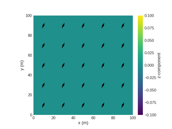
Visualising the field using matplotlib.

>>> import discretisedfield as df
...
>>> p1 = (0, 0, 0)
>>> p2 = (100, 100, 100)
>>> n = (10, 10, 10)
>>> mesh = df.Mesh(p1=p1, p2=p2, n=n)
>>> field = df.Field(mesh, nvdim=3, value=(1, 2, 0))
>>> field.sel(z=50).resample(n=(5, 5)).mpl()

../../_images/discretisedfield-Field-1.png

property norm#

Norm of the field.

Computes the norm of the field and returns discretisedfield.Field with nvdim=1. Norm of a scalar field is interpreted as an absolute value of the field.

The field norm can be set by passing numbers.Real, numpy.ndarray, or callable. If the field contains zero values, norm cannot be set and ValueError is raised.

Parameters:

numbers.Real – Norm value.
numpy.ndarray – Norm value.
callable – Norm value.

Returns:

Norm of the field.

Return type:

discretisedfield.Field

Raises:

ValueError – If the norm is set with wrong type, shape, or value. In addition, if the field contains zero values.

Examples

Manipulating the field norm.

>>> import discretisedfield as df
...
>>> p1 = (0, 0, 0)
>>> p2 = (1, 1, 1)
>>> cell = (1, 1, 1)
>>> mesh = df.Mesh(region=df.Region(p1=p1, p2=p2), cell=cell)
...
>>> field = df.Field(mesh=mesh, nvdim=3, value=(0, 0, 1))
>>> field.norm
Field(...)
>>> field.norm.mean()
array([1.])
>>> field.norm = 2
>>> field.mean()
array([0., 0., 2.])
>>> field.update_field_values((1, 0, 0))
>>> field.norm.mean()
array([1.])

Set the norm for a zero field. >>> field.update_field_values(0) >>> field.mean() array([0., 0., 0.]) >>> field.norm = 1 >>> field.mean() array([0., 0., 0.])

See also

__abs__()

property nvdim#

Number of value dimensions.

Returns:: Scalar fields have dimension 1, vector fields can have any dimension greater than 1.
Return type:: int

property orientation#

Orientation field.

This method computes the orientation (direction) of a vector field and returns discretisedfield.Field with the same dimension. More precisely, at every mesh discretisation cell, the vector is divided by its norm, so that a unit vector is obtained. However, if the vector at a discretisation cell is a zero-vector, it remains unchanged. In the case of a scalar (nvdim=1) field, ValueError is raised.

Returns:: Orientation field.
Return type:: discretisedfield.Field

Examples

Computing the orientation field.

>>> import discretisedfield as df
...
>>> p1 = (0, 0, 0)
>>> p2 = (10, 10, 10)
>>> cell = (1, 1, 1)
>>> mesh = df.Mesh(p1=p1, p2=p2, cell=cell)
...
>>> field = df.Field(mesh=mesh, nvdim=3, value=(6, 0, 8))
>>> field.orientation
Field(...)
>>> field.orientation.norm.mean()
array([1.])

property phase#: Phase of complex field.

property real#: Real part of complex field.

property unit#

Unit of the field.

Returns:: The unit of the field.
Return type:: str

property valid#

Valid field values.

This property is used to mask invalid field values. This can be achieved by passing numpy.ndarray of the same shape as the field array with boolean values, the string "norm" (which masks zero values), or None (which sets all values to True).

property vdim_mapping#: Map vdims to dims.

property vdims#: Vector components of the field.