Current induced domain wall motion using STT#
Problem description#
In this tutorial we show how Zhang-Li spin transfer torque (STT) can be included in micromagnetic simulations. To illustrate that, we will try to move a domain wall pair using spin-polarised current.
Let us simulate a two-dimensional sample with length \(L = 500 \,\text{nm}\), width \(w = 20 \,\text{nm}\) and discretisation cell \((2.5 \,\text{nm}, 2.5 \,\text{nm}, 2.5 \,\text{nm})\). The material parameters are:
exchange energy constant \(A = 15 \,\text{pJ}\,\text{m}^{-1}\),
Dzyaloshinskii-Moriya energy constant \(D = 3 \,\text{mJ}\,\text{m}^{-2}\),
uniaxial anisotropy constant \(K = 0.5 \,\text{MJ}\,\text{m}^{-3}\) with easy axis \(\mathbf{u}\) in the out of plane direction \((0, 0, 1)\),
gyrotropic ratio \(\gamma = 2.211 \times 10^{5} \,\text{m}\,\text{A}^{-1}\,\text{s}^{-1}\), and
Gilbert damping \(\alpha=0.3\).
Domain-wall pair#
[1]:
import oommfc as mc
import discretisedfield as df
import micromagneticmodel as mm

# Definition of parameters
L = 500e-9  # sample length (m)
w = 20e-9  # sample width (m)
d = 2.5e-9  # discretisation cell size (m)
Ms = 5.8e5  # saturation magnetisation (A/m)
A = 15e-12  # exchange energy constant (J/)
D = 3e-3  # Dzyaloshinkii-Moriya energy constant (J/m**2)
K = 0.5e6  # uniaxial anisotropy constant (J/m**3)
u = (0, 0, 1)  # easy axis
gamma0 = 2.211e5  # gyromagnetic ratio (m/As)
alpha = 0.3  # Gilbert damping

# Mesh definition
p1 = (0, 0, 0)
p2 = (L, w, d)
cell = (d, d, d)
region = df.Region(p1=p1, p2=p2)
mesh = df.Mesh(region=region, cell=cell)

# Micromagnetic system definition
system = mm.System(name="domain_wall_pair")
system.energy = (
    mm.Exchange(A=A)
    + mm.DMI(D=D, crystalclass="Cnv_z")
    + mm.UniaxialAnisotropy(K=K, u=u)
)
system.dynamics = mm.Precession(gamma0=gamma0) + mm.Damping(alpha=alpha)
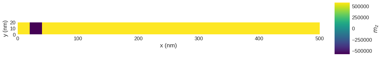
Because we want to move a DW pair, we need to initialise the magnetisation in an appropriate way before we relax the system.
[2]:
def m_value(pos):
    x, y, z = pos
    if 20e-9 < x < 40e-9:
        return (0, 0, -1)
    else:
        return (0, 0, 1)


system.m = df.Field(mesh, nvdim=3, value=m_value, norm=Ms)

system.m.z.sel("z").mpl(scalar_kw={"colorbar_label": "$m_z$"}, figsize=(15, 10))
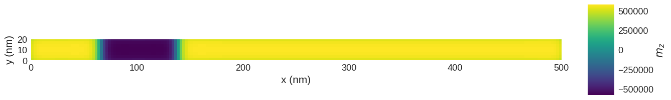
Now, we can relax the magnetisation.
[3]:
md = mc.MinDriver()
md.drive(system)
Running OOMMF (ExeOOMMFRunner)[2023/10/23 16:04]... (8.5 s)
[4]:
system.m.z.sel("z").mpl(scalar_kw={"colorbar_label": "$m_z$"}, figsize=(15, 10))
Now we can add the STT term to the dynamics equation.
[5]:
ux = 400  # velocity in x-direction (m/s)
beta = 0.5  # non-adiabatic STT parameter

system.dynamics += mm.ZhangLi(u=ux, beta=beta)  # please notice the use of `+=` operator
And drive the system for \(0.5 \,\text{ns}\):
[6]:
td = mc.TimeDriver()
td.drive(system, t=0.5e-9, n=100)
Running OOMMF (ExeOOMMFRunner)[2023/10/23 16:05]... (4.2 s)
[7]:
system.m.z.sel("z").mpl(scalar_kw={"colorbar_label": "$m_z$"}, figsize=(15, 10))
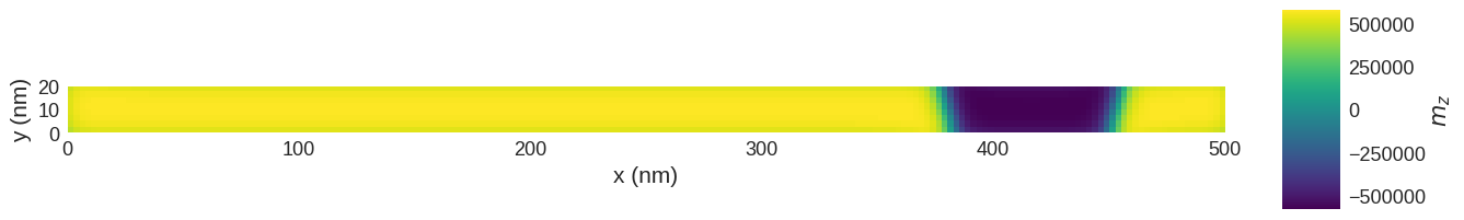
We see that the DW pair has moved to the positive \(x\) direction. Now, let us visualise the motion using interactive plot.
[8]:
import micromagneticdata as md

data = md.Data(system.name)
[9]:
data[1].hv(kdims=["x", "y"])
[9]:
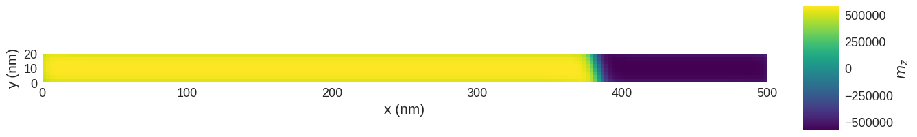
Single domain wall#
Modify the previous code to obtain one domain wall instead of a domain wall pair and move it using the same current.
Solution
[10]:
# Definition of parameters
L = 500e-9 # sample length (m)
w = 20e-9 # sample width (m)
d = 2.5e-9 # discretisation cell size (m)
Ms = 5.8e5 # saturation magnetisation (A/m)
A = 15e-12 # exchange energy constant (J/)
D = 3e-3 # Dzyaloshinkii-Moriya energy constant (J/m**2)
K = 0.5e6 # uniaxial anisotropy constant (J/m**3)
u = (0, 0, 1) # easy axis
gamma0 = 2.211e5 # gyromagnetic ratio (m/As)
alpha = 0.3 # Gilbert damping
# Mesh definition
p1 = (0, 0, 0)
p2 = (L, w, d)
cell = (d, d, d)
region = df.Region(p1=p1, p2=p2)
mesh = df.Mesh(region=region, cell=cell)
# Micromagnetic system definition
system = mm.System(name="domain_wall")
system.energy = (
mm.Exchange(A=A)
+ mm.DMI(D=D, crystalclass="Cnv_z")
+ mm.UniaxialAnisotropy(K=K, u=u)
)
system.dynamics = mm.Precession(gamma0=gamma0) + mm.Damping(alpha=alpha)
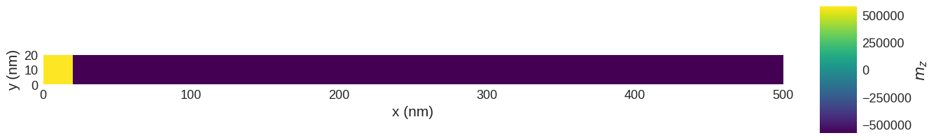
def m_value(pos):
x, y, z = pos
# Modify the following line
if 20e-9 < x:
return (0, 0, -1)
else:
return (0, 0, 1)
# We have added the y-component of 1e-8 to the magnetisation to be able to
# plot the vector field. This will not be necessary in the long run.
system.m = df.Field(mesh, nvdim=3, value=m_value, norm=Ms)
[11]:
system.m.z.sel("z").mpl(scalar_kw={"colorbar_label": "$m_z$"}, figsize=(15, 10))
[12]:
md = mc.MinDriver()
md.drive(system)
Running OOMMF (ExeOOMMFRunner)[2023/10/23 16:05]... (4.2 s)
[13]:
system.m.z.sel("z").mpl(scalar_kw={"colorbar_label": "$m_z$"}, figsize=(15, 10))
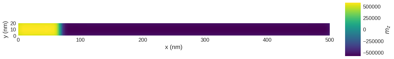
[14]:
ux = 400  # velocity in x direction (m/s)
beta = 0.5  # non-adiabatic STT parameter

system.dynamics += mm.ZhangLi(u=ux, beta=beta)

td = mc.TimeDriver()
td.drive(system, t=0.5e-9, n=100)
Running OOMMF (ExeOOMMFRunner)[2023/10/23 16:05]... (3.8 s)
[15]:
system.m.z.sel("z").mpl(scalar_kw={"colorbar_label": "$m_z$"}, figsize=(15, 10))