Field Valid

The discretisedfield.Field class features a valid property, specifically designed to indicate which values within a field should be considered during specific operations and which ones should be disregarded. While not all functions recognize the valid property, it plays a pivotal role in tasks such as plotting and differentiation.

In this tutorial, we will delve into the various methods to set the valid property and shed light on its applications. To illustrate its functionality, we will create a scalar field on a 2D mesh and examine how valid operates within this context.

import numpy as np

import discretisedfield as df

mesh = df.Mesh(p1=(0, 0), p2=(2, 2), n=(2, 2))

When initializing our field, we can provide an argument named valid. By default, this argument is set to True, ensuring the field is valid everywhere.

field = df.Field(mesh, nvdim=1, value=1)
field.valid

array([[ True,  True],
       [ True,  True]])

We can also explicitly set the valid property using a boolean value, either True or False, to indicate the field’s validity status.

field = df.Field(mesh, nvdim=1, value=1, valid=True)
field.valid

array([[ True,  True],
       [ True,  True]])

In fact, we can actually set valid using the exact same methods that we use to set the field values. For more information on ways this can be set please refer to the spatially varying fields notebook.

Let us try to set valid with a multidimensional list.

valid = [[True, True], [True, False]]
field_2 = df.Field(mesh, nvdim=1, value=1, valid=valid)
field_2.valid

array([[ True,  True],
       [ True, False]])

Plotting

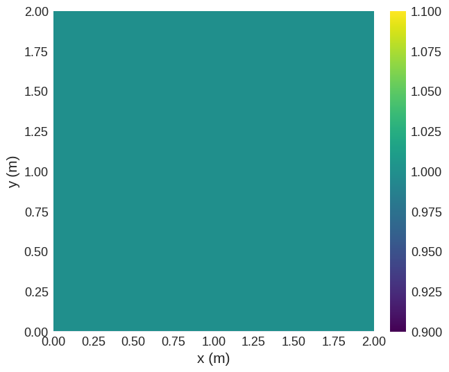
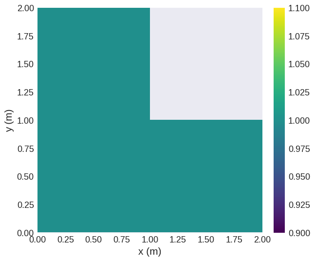
One of the functions that utilises valid is plotting. When plotting both fields we can see that any cell which has valid=False is masked.

field.mpl()

field_2.mpl()

Even after initialization, the valid property remains flexible, allowing for subsequent modifications.

field_2.valid = True
field_2.valid

array([[ True,  True],
       [ True,  True]])

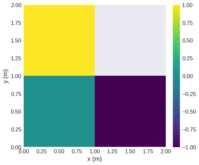
Besides the conventional methods to set field values, the valid property can also automatically be set based on the norm of the field values. This can be achieved by passing "norm" to valid.

value = np.array([[[0, 1, 0], [0, 1, 1]], [[0, 1, -1], [0, 0, 0]]])
field_3 = df.Field(mesh, nvdim=3, value=value, valid="norm")
field_3.valid

array([[ True,  True],
       [ True, False]])

field_3.z.mpl()

Operations

Operations can be performed between fields with different valid attributes but special attention must be given to ensure that the resulting field also accurately represents its validity. When you perform an operation on these fields, the resulting valid attribute is determined by the logical AND operation on the valid attribute of the initial fields. This is performed element-wise on the arrays to find the intersection between them. Hence, for an element of the result to be True, both A and B must have valid attributes of True.

(field + field_3).valid

array([[ True,  True],
       [ True, False]])

The valid functionality is also used in other areas of discretisedfield such as differentiation. However, it is not used in all operations - for example fftn. Please refer to the API documentation for details on specific operations.