Analysing simulation results

With micromagneticdata we can analyse simulation results created with oommfc. This notebook summarises the available functionality.

import os

import micromagneticdata as md

We have a set of example simulations stored in the test directory of micromagneticdata that we use to demonstrate its functionality.

dirname = os.path.join("..", "micromagneticdata", "tests", "test_sample")

Data

First, we creata a Data object. We need to pass the name of the micromagneticmodel.System that we used to run the simulation and optionally an additional path to the base directory.

data = md.Data(name="rectangle", dirname=dirname)

The Data object contains all simulation runs of the System. These are called drives.

data.n

7

data.info

	drive_number	date	time	start_time	adapter	adapter_version	driver	t	n	end_time	elapsed_time	success	info.json	output_step
0	0	2025-05-31	22:02:42	2025-05-31T22:02:42	oommfc	0.65.0	TimeDriver	0.0	25	2025-05-31T22:02:42	00:00:01	True	available	<NA>
1	1	2025-05-31	22:02:42	2025-05-31T22:02:42	mumax3c	0.3.0	TimeDriver	0.0	15	2025-05-31T22:02:42	00:00:01	True	available	<NA>
2	2	2025-05-31	22:02:42	2025-05-31T22:02:42	mumax3c	0.3.0	TimeDriver	0.0	250	2025-05-31T22:02:43	00:00:01	True	available	<NA>
3	3	2025-05-31	22:02:43	2025-05-31T22:02:43	mumax3c	0.3.0	RelaxDriver	<NA>	<NA>	2025-05-31T22:02:43	00:00:01	True	available	<NA>
4	4	2025-05-31	22:02:43	2025-05-31T22:02:43	mumax3c	0.3.0	MinDriver	<NA>	<NA>	2025-05-31T22:02:43	00:00:01	True	available	<NA>
5	5	2025-05-31	22:02:43	2025-05-31T22:02:43	oommfc	0.65.0	TimeDriver	0.0	5	2025-05-31T22:02:44	00:00:01	True	available	<NA>
6	6	2025-05-31	22:02:44	2025-05-31T22:02:44	oommfc	0.65.0	MinDriver	<NA>	<NA>	2025-05-31T22:02:44	00:00:01	True	available	True

Drive

To access one Drive we can index the Data object.

drive = data[6]

The Drive object has a number of properties containing information about the drive.

drive.n

14

drive.info

{'drive_number': 6,
 'date': '2025-05-31',
 'time': '22:02:44',
 'start_time': '2025-05-31T22:02:44',
 'adapter': 'oommfc',
 'adapter_version': '0.65.0',
 'driver': 'MinDriver',
 'output_step': True,
 'end_time': '2025-05-31T22:02:44',
 'elapsed_time': '00:00:01',
 'success': True}

drive = data[6]

drive.x

'iteration'

drive.info

{'drive_number': 6,
 'date': '2025-05-31',
 'time': '22:02:44',
 'start_time': '2025-05-31T22:02:44',
 'adapter': 'oommfc',
 'adapter_version': '0.65.0',
 'driver': 'MinDriver',
 'output_step': True,
 'end_time': '2025-05-31T22:02:44',
 'elapsed_time': '00:00:01',
 'success': True}

print(drive.calculator_script)

# MIF 2.2

SetOptions {
  basename rectangle
  scalar_output_format %.12g
  scalar_field_output_format {binary 8}
  vector_field_output_format {binary 8}
}

# BoxAtlas for total_atlas
Specify Oxs_BoxAtlas:total_atlas {
  xrange { -5e-08 5e-08 }
  yrange { -2.5e-08 2.5e-08 }
  zrange { 0.0 2e-08 }
  name total
}

# BoxAtlas for entire_atlas
Specify Oxs_BoxAtlas:entire_atlas {
  xrange { -5e-08 5e-08 }
  yrange { -2.5e-08 2.5e-08 }
  zrange { 0.0 2e-08 }
  name entire
}

# MultiAtlas
Specify Oxs_MultiAtlas:main_atlas {
  atlas :total_atlas
  atlas :entire_atlas
  xrange { -5e-08 5e-08 }
  yrange { -2.5e-08 2.5e-08 }
  zrange { 0.0 2e-08 }
}

# RectangularMesh
Specify Oxs_RectangularMesh:mesh {
  cellsize { 5e-09 5e-09 5e-09 }
  atlas :main_atlas
}

# UniformExchange
Specify Oxs_UniformExchange:exchange {
  A 1.3e-11
}

# FixedZeeman
Specify Oxs_FixedZeeman:zeeman {
  field {0.0 0.0 1000000.0}
}

# m0 file
Specify Oxs_FileVectorField:m0 {
  file m0.omf
  atlas :main_atlas
}

# m0_norm
Specify Oxs_VecMagScalarField:m0_norm {
    field :m0
}

# CGEvolver
Specify Oxs_CGEvolve:evolver {
}

# MinDriver
Specify Oxs_MinDriver {
  evolver :evolver
  mesh :mesh
  Ms :m0_norm
  m0 :m0
  stopping_mxHxm 0.1
}

Destination table mmArchive
Destination mags mmArchive

Schedule DataTable table Step 1
Schedule Oxs_MinDriver::Magnetization mags Step 1

The initial magnetisation can be obtained with m0. It returns a discretisedfield.Field object.

drive.m0

Field

• Mesh
  • Region
    • pmin = [-5e-08, -2.5e-08, 0.0]
    • pmax = [5e-08, 2.5e-08, 2e-08]
    • dims = ['x', 'y', 'z']
    • units = ['m', 'm', 'm']
  • n = [20, 10, 4]
  • subregions:
    • Region total
      • pmin = [-5e-08, -2.5e-08, 0.0]
      • pmax = [5e-08, 2.5e-08, 2e-08]
      • dims = ['x', 'y', 'z']
      • units = ['m', 'm', 'm']
• nvdim = 3
• vdims:
  • x
  • y
  • z
• unit = None

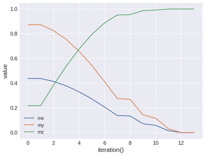
Scalar data of the drive can be accessed via the table property that returns a ubermagtable.Table object.

drive.table.mpl(y=["mx", "my", "mz"])

drive.n

14

We can access the magnetisation at a single step or iterate over the drive.

drive[0]

Field

• Mesh
  • Region
    • pmin = [-5e-08, -2.5e-08, 0.0]
    • pmax = [5e-08, 2.5e-08, 2e-08]
    • dims = ['x', 'y', 'z']
    • units = ['m', 'm', 'm']
  • n = [20, 10, 4]
  • subregions:
    • Region total
      • pmin = [-5e-08, -2.5e-08, 0.0]
      • pmax = [5e-08, 2.5e-08, 2e-08]
      • dims = ['x', 'y', 'z']
      • units = ['m', 'm', 'm']
• nvdim = 3
• vdims:
  • x
  • y
  • z
• unit = A/m

list(drive)

[Field(Mesh(Region(pmin=[-5e-08, -2.5e-08, 0.0], pmax=[5e-08, 2.5e-08, 2e-08], dims=['x', 'y', 'z'], units=['m', 'm', 'm']), n=[20, 10, 4], subregions: (Region`total`(pmin=[-5e-08, -2.5e-08, 0.0], pmax=[5e-08, 2.5e-08, 2e-08], dims=['x', 'y', 'z'], units=['m', 'm', 'm']))), nvdim=3, vdims: (x, y, z), unit=A/m),
 Field(Mesh(Region(pmin=[-5e-08, -2.5e-08, 0.0], pmax=[5e-08, 2.5e-08, 2e-08], dims=['x', 'y', 'z'], units=['m', 'm', 'm']), n=[20, 10, 4], subregions: (Region`total`(pmin=[-5e-08, -2.5e-08, 0.0], pmax=[5e-08, 2.5e-08, 2e-08], dims=['x', 'y', 'z'], units=['m', 'm', 'm']))), nvdim=3, vdims: (x, y, z), unit=A/m),
 Field(Mesh(Region(pmin=[-5e-08, -2.5e-08, 0.0], pmax=[5e-08, 2.5e-08, 2e-08], dims=['x', 'y', 'z'], units=['m', 'm', 'm']), n=[20, 10, 4], subregions: (Region`total`(pmin=[-5e-08, -2.5e-08, 0.0], pmax=[5e-08, 2.5e-08, 2e-08], dims=['x', 'y', 'z'], units=['m', 'm', 'm']))), nvdim=3, vdims: (x, y, z), unit=A/m),
 Field(Mesh(Region(pmin=[-5e-08, -2.5e-08, 0.0], pmax=[5e-08, 2.5e-08, 2e-08], dims=['x', 'y', 'z'], units=['m', 'm', 'm']), n=[20, 10, 4], subregions: (Region`total`(pmin=[-5e-08, -2.5e-08, 0.0], pmax=[5e-08, 2.5e-08, 2e-08], dims=['x', 'y', 'z'], units=['m', 'm', 'm']))), nvdim=3, vdims: (x, y, z), unit=A/m),
 Field(Mesh(Region(pmin=[-5e-08, -2.5e-08, 0.0], pmax=[5e-08, 2.5e-08, 2e-08], dims=['x', 'y', 'z'], units=['m', 'm', 'm']), n=[20, 10, 4], subregions: (Region`total`(pmin=[-5e-08, -2.5e-08, 0.0], pmax=[5e-08, 2.5e-08, 2e-08], dims=['x', 'y', 'z'], units=['m', 'm', 'm']))), nvdim=3, vdims: (x, y, z), unit=A/m),
 Field(Mesh(Region(pmin=[-5e-08, -2.5e-08, 0.0], pmax=[5e-08, 2.5e-08, 2e-08], dims=['x', 'y', 'z'], units=['m', 'm', 'm']), n=[20, 10, 4], subregions: (Region`total`(pmin=[-5e-08, -2.5e-08, 0.0], pmax=[5e-08, 2.5e-08, 2e-08], dims=['x', 'y', 'z'], units=['m', 'm', 'm']))), nvdim=3, vdims: (x, y, z), unit=A/m),
 Field(Mesh(Region(pmin=[-5e-08, -2.5e-08, 0.0], pmax=[5e-08, 2.5e-08, 2e-08], dims=['x', 'y', 'z'], units=['m', 'm', 'm']), n=[20, 10, 4], subregions: (Region`total`(pmin=[-5e-08, -2.5e-08, 0.0], pmax=[5e-08, 2.5e-08, 2e-08], dims=['x', 'y', 'z'], units=['m', 'm', 'm']))), nvdim=3, vdims: (x, y, z), unit=A/m),
 Field(Mesh(Region(pmin=[-5e-08, -2.5e-08, 0.0], pmax=[5e-08, 2.5e-08, 2e-08], dims=['x', 'y', 'z'], units=['m', 'm', 'm']), n=[20, 10, 4], subregions: (Region`total`(pmin=[-5e-08, -2.5e-08, 0.0], pmax=[5e-08, 2.5e-08, 2e-08], dims=['x', 'y', 'z'], units=['m', 'm', 'm']))), nvdim=3, vdims: (x, y, z), unit=A/m),
 Field(Mesh(Region(pmin=[-5e-08, -2.5e-08, 0.0], pmax=[5e-08, 2.5e-08, 2e-08], dims=['x', 'y', 'z'], units=['m', 'm', 'm']), n=[20, 10, 4], subregions: (Region`total`(pmin=[-5e-08, -2.5e-08, 0.0], pmax=[5e-08, 2.5e-08, 2e-08], dims=['x', 'y', 'z'], units=['m', 'm', 'm']))), nvdim=3, vdims: (x, y, z), unit=A/m),
 Field(Mesh(Region(pmin=[-5e-08, -2.5e-08, 0.0], pmax=[5e-08, 2.5e-08, 2e-08], dims=['x', 'y', 'z'], units=['m', 'm', 'm']), n=[20, 10, 4], subregions: (Region`total`(pmin=[-5e-08, -2.5e-08, 0.0], pmax=[5e-08, 2.5e-08, 2e-08], dims=['x', 'y', 'z'], units=['m', 'm', 'm']))), nvdim=3, vdims: (x, y, z), unit=A/m),
 Field(Mesh(Region(pmin=[-5e-08, -2.5e-08, 0.0], pmax=[5e-08, 2.5e-08, 2e-08], dims=['x', 'y', 'z'], units=['m', 'm', 'm']), n=[20, 10, 4], subregions: (Region`total`(pmin=[-5e-08, -2.5e-08, 0.0], pmax=[5e-08, 2.5e-08, 2e-08], dims=['x', 'y', 'z'], units=['m', 'm', 'm']))), nvdim=3, vdims: (x, y, z), unit=A/m),
 Field(Mesh(Region(pmin=[-5e-08, -2.5e-08, 0.0], pmax=[5e-08, 2.5e-08, 2e-08], dims=['x', 'y', 'z'], units=['m', 'm', 'm']), n=[20, 10, 4], subregions: (Region`total`(pmin=[-5e-08, -2.5e-08, 0.0], pmax=[5e-08, 2.5e-08, 2e-08], dims=['x', 'y', 'z'], units=['m', 'm', 'm']))), nvdim=3, vdims: (x, y, z), unit=A/m),
 Field(Mesh(Region(pmin=[-5e-08, -2.5e-08, 0.0], pmax=[5e-08, 2.5e-08, 2e-08], dims=['x', 'y', 'z'], units=['m', 'm', 'm']), n=[20, 10, 4], subregions: (Region`total`(pmin=[-5e-08, -2.5e-08, 0.0], pmax=[5e-08, 2.5e-08, 2e-08], dims=['x', 'y', 'z'], units=['m', 'm', 'm']))), nvdim=3, vdims: (x, y, z), unit=A/m),
 Field(Mesh(Region(pmin=[-5e-08, -2.5e-08, 0.0], pmax=[5e-08, 2.5e-08, 2e-08], dims=['x', 'y', 'z'], units=['m', 'm', 'm']), n=[20, 10, 4], subregions: (Region`total`(pmin=[-5e-08, -2.5e-08, 0.0], pmax=[5e-08, 2.5e-08, 2e-08], dims=['x', 'y', 'z'], units=['m', 'm', 'm']))), nvdim=3, vdims: (x, y, z), unit=A/m)]

We can also select a parts of the data and get a new drive, e.g. every second of the first 10 elements.

drive_selection = drive[:10:2]
drive_selection

OOMMFDrive(name='rectangle', number=6, dirname='../micromagneticdata/tests/test_sample', x='iteration')

drive_selection.n

5

It is possible to convert all magnetisation files into vtk for visualisation e.g. in Paraview.

# drive.ovf2vtk()

We can convert a drive into an xarray.DataArray. An additional dimension is added depending on the type of drive.

drive.to_xarray()

<xarray.DataArray 'field' (iteration: 14, x: 20, y: 10, z: 4, vdims: 3)>
array([[[[[ 3.50067876e+05,  6.98022376e+05,  1.73831082e+05],
          [ 3.50067876e+05,  6.98022376e+05,  1.73831082e+05],
          [ 3.50067876e+05,  6.98022376e+05,  1.73831082e+05],
          [ 3.50067876e+05,  6.98022376e+05,  1.73831082e+05]],

         [[ 3.50067876e+05,  6.98022376e+05,  1.73831082e+05],
          [ 3.50067876e+05,  6.98022376e+05,  1.73831082e+05],
          [ 3.50067876e+05,  6.98022376e+05,  1.73831082e+05],
          [ 3.50067876e+05,  6.98022376e+05,  1.73831082e+05]],

         [[ 3.50067876e+05,  6.98022376e+05,  1.73831082e+05],
          [ 3.50067876e+05,  6.98022376e+05,  1.73831082e+05],
          [ 3.50067876e+05,  6.98022376e+05,  1.73831082e+05],
          [ 3.50067876e+05,  6.98022376e+05,  1.73831082e+05]],

         ...,

         [[ 3.50067876e+05,  6.98022376e+05,  1.73831082e+05],
          [ 3.50067876e+05,  6.98022376e+05,  1.73831082e+05],
          [ 3.50067876e+05,  6.98022376e+05,  1.73831082e+05],
...
          [-3.41568167e-06, -6.81074074e-06,  8.00000000e+05],
          [-3.41568167e-06, -6.81074074e-06,  8.00000000e+05],
          [-3.41568167e-06, -6.81074074e-06,  8.00000000e+05]],

         ...,

         [[-3.41568167e-06, -6.81074074e-06,  8.00000000e+05],
          [-3.41568167e-06, -6.81074074e-06,  8.00000000e+05],
          [-3.41568167e-06, -6.81074074e-06,  8.00000000e+05],
          [-3.41568167e-06, -6.81074074e-06,  8.00000000e+05]],

         [[-3.41568167e-06, -6.81074074e-06,  8.00000000e+05],
          [-3.41568167e-06, -6.81074074e-06,  8.00000000e+05],
          [-3.41568167e-06, -6.81074074e-06,  8.00000000e+05],
          [-3.41568167e-06, -6.81074074e-06,  8.00000000e+05]],

         [[-3.41568167e-06, -6.81074074e-06,  8.00000000e+05],
          [-3.41568167e-06, -6.81074074e-06,  8.00000000e+05],
          [-3.41568167e-06, -6.81074074e-06,  8.00000000e+05],
          [-3.41568167e-06, -6.81074074e-06,  8.00000000e+05]]]]])
Coordinates:
  * x          (x) float64 -4.75e-08 -4.25e-08 -3.75e-08 ... 4.25e-08 4.75e-08
  * y          (y) float64 -2.25e-08 -1.75e-08 -1.25e-08 ... 1.75e-08 2.25e-08
  * z          (z) float64 2.5e-09 7.5e-09 1.25e-08 1.75e-08
  * vdims      (vdims) <U1 'x' 'y' 'z'
  * iteration  (iteration) float64 0.0 1.0 2.0 3.0 4.0 ... 10.0 11.0 12.0 13.0
Attributes:
    drive_number:     6
    date:             2025-05-31
    time:             22:02:44
    start_time:       2025-05-31T22:02:44
    adapter:          oommfc
    adapter_version:  0.65.0
    driver:           MinDriver
    output_step:      True
    end_time:         2025-05-31T22:02:44
    elapsed_time:     00:00:01
    success:          True

xarray.DataArray

'field'

• iteration: 14
• x: 20
• y: 10
• z: 4
• vdims: 3

• 3.501e+05 6.98e+05 1.738e+05 3.501e+05 ... -3.416e-06 -6.811e-06 8e+05

  array([[[[[ 3.50067876e+05,  6.98022376e+05,  1.73831082e+05],
            [ 3.50067876e+05,  6.98022376e+05,  1.73831082e+05],
            [ 3.50067876e+05,  6.98022376e+05,  1.73831082e+05],
            [ 3.50067876e+05,  6.98022376e+05,  1.73831082e+05]],
  
           [[ 3.50067876e+05,  6.98022376e+05,  1.73831082e+05],
            [ 3.50067876e+05,  6.98022376e+05,  1.73831082e+05],
            [ 3.50067876e+05,  6.98022376e+05,  1.73831082e+05],
            [ 3.50067876e+05,  6.98022376e+05,  1.73831082e+05]],
  
           [[ 3.50067876e+05,  6.98022376e+05,  1.73831082e+05],
            [ 3.50067876e+05,  6.98022376e+05,  1.73831082e+05],
            [ 3.50067876e+05,  6.98022376e+05,  1.73831082e+05],
            [ 3.50067876e+05,  6.98022376e+05,  1.73831082e+05]],
  
           ...,
  
           [[ 3.50067876e+05,  6.98022376e+05,  1.73831082e+05],
            [ 3.50067876e+05,  6.98022376e+05,  1.73831082e+05],
            [ 3.50067876e+05,  6.98022376e+05,  1.73831082e+05],
  ...
            [-3.41568167e-06, -6.81074074e-06,  8.00000000e+05],
            [-3.41568167e-06, -6.81074074e-06,  8.00000000e+05],
            [-3.41568167e-06, -6.81074074e-06,  8.00000000e+05]],
  
           ...,
  
           [[-3.41568167e-06, -6.81074074e-06,  8.00000000e+05],
            [-3.41568167e-06, -6.81074074e-06,  8.00000000e+05],
            [-3.41568167e-06, -6.81074074e-06,  8.00000000e+05],
            [-3.41568167e-06, -6.81074074e-06,  8.00000000e+05]],
  
           [[-3.41568167e-06, -6.81074074e-06,  8.00000000e+05],
            [-3.41568167e-06, -6.81074074e-06,  8.00000000e+05],
            [-3.41568167e-06, -6.81074074e-06,  8.00000000e+05],
            [-3.41568167e-06, -6.81074074e-06,  8.00000000e+05]],
  
           [[-3.41568167e-06, -6.81074074e-06,  8.00000000e+05],
            [-3.41568167e-06, -6.81074074e-06,  8.00000000e+05],
            [-3.41568167e-06, -6.81074074e-06,  8.00000000e+05],
            [-3.41568167e-06, -6.81074074e-06,  8.00000000e+05]]]]])

• Coordinates: (5)
  • x
    (x)
    float64
    -4.75e-08 -4.25e-08 ... 4.75e-08

    units :

    m

    array([-4.75e-08, -4.25e-08, -3.75e-08, -3.25e-08, -2.75e-08, -2.25e-08,
           -1.75e-08, -1.25e-08, -7.50e-09, -2.50e-09,  2.50e-09,  7.50e-09,
            1.25e-08,  1.75e-08,  2.25e-08,  2.75e-08,  3.25e-08,  3.75e-08,
            4.25e-08,  4.75e-08])

  • y
    (y)
    float64
    -2.25e-08 -1.75e-08 ... 2.25e-08

    units :

    m

    array([-2.25e-08, -1.75e-08, -1.25e-08, -7.50e-09, -2.50e-09,  2.50e-09,
            7.50e-09,  1.25e-08,  1.75e-08,  2.25e-08])

  • z
    (z)
    float64
    2.5e-09 7.5e-09 1.25e-08 1.75e-08

    units :

    m

    array([2.50e-09, 7.50e-09, 1.25e-08, 1.75e-08])

  • vdims
    (vdims)
    <U1
    'x' 'y' 'z'

    array(['x', 'y', 'z'], dtype='<U1')

  • iteration
    (iteration)
    float64
    0.0 1.0 2.0 3.0 ... 11.0 12.0 13.0

    units :

    array([ 0.,  1.,  2.,  3.,  4.,  5.,  6.,  7.,  8.,  9., 10., 11., 12., 13.])

• Indexes: (5)
  • x
    PandasIndex

    PandasIndex(Index([-4.7499999999999995e-08,               -4.25e-08,
                         -3.75e-08,  -3.249999999999999e-08,
           -2.7499999999999998e-08,               -2.25e-08,
           -1.7499999999999998e-08,               -1.25e-08,
            -7.500000000000001e-09, -2.5000000000000025e-09,
             2.499999999999996e-09,   7.499999999999994e-09,
                          1.25e-08,   1.749999999999999e-08,
            2.2499999999999996e-08,  2.7499999999999988e-08,
             3.249999999999999e-08,                3.75e-08,
             4.249999999999999e-08,  4.7499999999999995e-08],
          dtype='float64', name='x'))

  • y
    PandasIndex

    PandasIndex(Index([              -2.25e-08, -1.7499999999999998e-08,
                         -1.25e-08,  -7.499999999999998e-09,
           -2.4999999999999992e-09,  2.4999999999999992e-09,
             7.500000000000004e-09,  1.2500000000000003e-08,
                          1.75e-08,                2.25e-08],
          dtype='float64', name='y'))

  • z
    PandasIndex

    PandasIndex(Index([2.5e-09, 7.500000000000001e-09, 1.2500000000000003e-08, 1.75e-08], dtype='float64', name='z'))

  • vdims
    PandasIndex

    PandasIndex(Index(['x', 'y', 'z'], dtype='object', name='vdims'))

  • iteration
    PandasIndex

    PandasIndex(Index([0.0, 1.0, 2.0, 3.0, 4.0, 5.0, 6.0, 7.0, 8.0, 9.0, 10.0, 11.0, 12.0,
           13.0],
          dtype='float64', name='iteration'))

• Attributes: (11)

  drive_number :

  6

  date :

  2025-05-31

  time :

  22:02:44

  start_time :

  2025-05-31T22:02:44

  adapter :

  oommfc

  adapter_version :

  0.65.0

  driver :

  MinDriver

  output_step :

  True

  end_time :

  2025-05-31T22:02:44

  elapsed_time :

  00:00:01

  success :

  True

CombinedDrive

Multiple drives can be concatenated to create one “longer” drive. This can e.g. be convenient to analyse multiple consecutive time drives. Combining drives is done via the << operator which appends the right-hand-side drive to the left-hand-side drive. It returns a new CombinedDrive object that behaves very similar to the Drive object.

combined = data[0] << data[1] << data[2]
combined

CombinedDrive(
  OOMMFDrive(name='rectangle', number=0, dirname='../micromagneticdata/tests/test_sample', x='t'),
  Mumax3Drive(name='rectangle', number=1, dirname='../micromagneticdata/tests/test_sample', x='t'),
  Mumax3Drive(name='rectangle', number=2, dirname='../micromagneticdata/tests/test_sample', x='t')
)

The combined drive has a property drives that provides a list of all individual drives.

combined.drives

(OOMMFDrive(name='rectangle', number=0, dirname='../micromagneticdata/tests/test_sample', x='t'),
 Mumax3Drive(name='rectangle', number=1, dirname='../micromagneticdata/tests/test_sample', x='t'),
 Mumax3Drive(name='rectangle', number=2, dirname='../micromagneticdata/tests/test_sample', x='t'))

combined.info

{'drive_numbers': [0, 1, 2], 'driver': 'TimeDriver'}

We have direct access to the initial magnetisation of the first drive.

combined.m0

Field

• Mesh
  • Region
    • pmin = [-5e-08, -2.5e-08, 0.0]
    • pmax = [5e-08, 2.5e-08, 2e-08]
    • dims = ['x', 'y', 'z']
    • units = ['m', 'm', 'm']
  • n = [20, 10, 4]
  • subregions:
    • Region total
      • pmin = [-5e-08, -2.5e-08, 0.0]
      • pmax = [5e-08, 2.5e-08, 2e-08]
      • dims = ['x', 'y', 'z']
      • units = ['m', 'm', 'm']
• nvdim = 3
• vdims:
  • x
  • y
  • z
• unit = None

combined.n

290

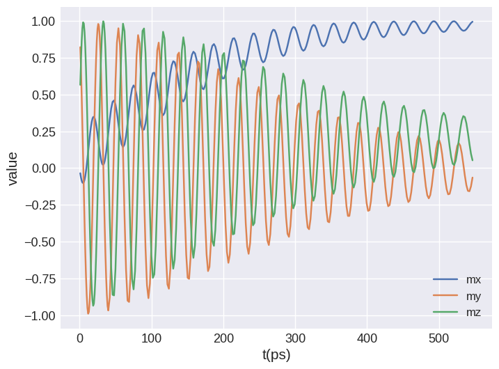
The combined drive has one large table that contains the data for all individual drives.

combined.table.mpl(y=["mx", "my", "mz"])

We can iterate over the drives in the combined drive or access a single element.

combined[15]

Field

• Mesh
  • Region
    • pmin = [-5e-08, -2.5e-08, 0.0]
    • pmax = [5e-08, 2.5e-08, 2e-08]
    • dims = ['x', 'y', 'z']
    • units = ['m', 'm', 'm']
  • n = [20, 10, 4]
  • subregions:
    • Region total
      • pmin = [-5e-08, -2.5e-08, 0.0]
      • pmax = [5e-08, 2.5e-08, 2e-08]
      • dims = ['x', 'y', 'z']
      • units = ['m', 'm', 'm']
• nvdim = 3
• vdims:
  • x
  • y
  • z
• unit = A/m

combined.x

't'

The combined drive can be converted into an xarray.DataArray similar to the normal Drive.

combined.to_xarray()

<xarray.DataArray 'field' (t: 290, x: 20, y: 10, z: 4, vdims: 3)>
array([[[[[ -27584.49540021,  658579.77501927,  453334.06616874],
          [ -27584.49540021,  658579.77501927,  453334.06616874],
          [ -27584.49540021,  658579.77501927,  453334.06616874],
          [ -27584.49540021,  658579.77501927,  453334.06616874]],

         [[ -27584.49540021,  658579.77501927,  453334.06616874],
          [ -27584.49540021,  658579.77501927,  453334.06616874],
          [ -27584.49540021,  658579.77501927,  453334.06616874],
          [ -27584.49540021,  658579.77501927,  453334.06616874]],

         [[ -27584.49540021,  658579.77501927,  453334.06616874],
          [ -27584.49540021,  658579.77501927,  453334.06616874],
          [ -27584.49540021,  658579.77501927,  453334.06616874],
          [ -27584.49540021,  658579.77501927,  453334.06616874]],

         ...,

         [[ -27584.49540021,  658579.77501927,  453334.06616874],
          [ -27584.49540021,  658579.77501927,  453334.06616874],
          [ -27584.49540021,  658579.77501927,  453334.06616874],
...
          [ 797212.875     ,  -51317.65625   ,   42639.36328125],
          [ 797212.875     ,  -51317.65625   ,   42639.36328125],
          [ 797212.875     ,  -51317.65625   ,   42639.36328125]],

         ...,

         [[ 797212.875     ,  -51317.65625   ,   42639.36328125],
          [ 797212.875     ,  -51317.65625   ,   42639.36328125],
          [ 797212.875     ,  -51317.65625   ,   42639.36328125],
          [ 797212.875     ,  -51317.65625   ,   42639.36328125]],

         [[ 797212.875     ,  -51317.65625   ,   42639.36328125],
          [ 797212.875     ,  -51317.65625   ,   42639.36328125],
          [ 797212.875     ,  -51317.65625   ,   42639.36328125],
          [ 797212.875     ,  -51317.65625   ,   42639.36328125]],

         [[ 797212.875     ,  -51317.65625   ,   42639.36328125],
          [ 797212.875     ,  -51317.65625   ,   42639.36328125],
          [ 797212.875     ,  -51317.65625   ,   42639.36328125],
          [ 797212.875     ,  -51317.65625   ,   42639.36328125]]]]])
Coordinates:
  * x        (x) float64 -4.75e-08 -4.25e-08 -3.75e-08 ... 4.25e-08 4.75e-08
  * y        (y) float64 -2.25e-08 -1.75e-08 -1.25e-08 ... 1.75e-08 2.25e-08
  * z        (z) float64 2.5e-09 7.5e-09 1.25e-08 1.75e-08
  * vdims    (vdims) <U1 'x' 'y' 'z'
  * t        (t) float64 1e-12 2e-12 3e-12 ... 5.423e-10 5.445e-10 5.466e-10
Attributes:
    drive_numbers:  [0, 1, 2]
    driver:         TimeDriver

xarray.DataArray

'field'

• t: 290
• x: 20
• y: 10
• z: 4
• vdims: 3

• -2.758e+04 6.586e+05 4.533e+05 ... 7.972e+05 -5.132e+04 4.264e+04

  array([[[[[ -27584.49540021,  658579.77501927,  453334.06616874],
            [ -27584.49540021,  658579.77501927,  453334.06616874],
            [ -27584.49540021,  658579.77501927,  453334.06616874],
            [ -27584.49540021,  658579.77501927,  453334.06616874]],
  
           [[ -27584.49540021,  658579.77501927,  453334.06616874],
            [ -27584.49540021,  658579.77501927,  453334.06616874],
            [ -27584.49540021,  658579.77501927,  453334.06616874],
            [ -27584.49540021,  658579.77501927,  453334.06616874]],
  
           [[ -27584.49540021,  658579.77501927,  453334.06616874],
            [ -27584.49540021,  658579.77501927,  453334.06616874],
            [ -27584.49540021,  658579.77501927,  453334.06616874],
            [ -27584.49540021,  658579.77501927,  453334.06616874]],
  
           ...,
  
           [[ -27584.49540021,  658579.77501927,  453334.06616874],
            [ -27584.49540021,  658579.77501927,  453334.06616874],
            [ -27584.49540021,  658579.77501927,  453334.06616874],
  ...
            [ 797212.875     ,  -51317.65625   ,   42639.36328125],
            [ 797212.875     ,  -51317.65625   ,   42639.36328125],
            [ 797212.875     ,  -51317.65625   ,   42639.36328125]],
  
           ...,
  
           [[ 797212.875     ,  -51317.65625   ,   42639.36328125],
            [ 797212.875     ,  -51317.65625   ,   42639.36328125],
            [ 797212.875     ,  -51317.65625   ,   42639.36328125],
            [ 797212.875     ,  -51317.65625   ,   42639.36328125]],
  
           [[ 797212.875     ,  -51317.65625   ,   42639.36328125],
            [ 797212.875     ,  -51317.65625   ,   42639.36328125],
            [ 797212.875     ,  -51317.65625   ,   42639.36328125],
            [ 797212.875     ,  -51317.65625   ,   42639.36328125]],
  
           [[ 797212.875     ,  -51317.65625   ,   42639.36328125],
            [ 797212.875     ,  -51317.65625   ,   42639.36328125],
            [ 797212.875     ,  -51317.65625   ,   42639.36328125],
            [ 797212.875     ,  -51317.65625   ,   42639.36328125]]]]])

• Coordinates: (5)
  • x
    (x)
    float64
    -4.75e-08 -4.25e-08 ... 4.75e-08

    units :

    m

    array([-4.75e-08, -4.25e-08, -3.75e-08, -3.25e-08, -2.75e-08, -2.25e-08,
           -1.75e-08, -1.25e-08, -7.50e-09, -2.50e-09,  2.50e-09,  7.50e-09,
            1.25e-08,  1.75e-08,  2.25e-08,  2.75e-08,  3.25e-08,  3.75e-08,
            4.25e-08,  4.75e-08])

  • y
    (y)
    float64
    -2.25e-08 -1.75e-08 ... 2.25e-08

    units :

    m

    array([-2.25e-08, -1.75e-08, -1.25e-08, -7.50e-09, -2.50e-09,  2.50e-09,
            7.50e-09,  1.25e-08,  1.75e-08,  2.25e-08])

  • z
    (z)
    float64
    2.5e-09 7.5e-09 1.25e-08 1.75e-08

    units :

    m

    array([2.50e-09, 7.50e-09, 1.25e-08, 1.75e-08])

  • vdims
    (vdims)
    <U1
    'x' 'y' 'z'

    array(['x', 'y', 'z'], dtype='<U1')

  • t
    (t)
    float64
    1e-12 2e-12 ... 5.445e-10 5.466e-10

    units :

    s

    array([1.000000e-12, 2.000000e-12, 3.000000e-12, ..., 5.423237e-10,
           5.444648e-10, 5.466095e-10])

• Indexes: (5)
  • x
    PandasIndex

    PandasIndex(Index([-4.7499999999999995e-08,               -4.25e-08,
                         -3.75e-08,  -3.249999999999999e-08,
           -2.7499999999999998e-08,               -2.25e-08,
           -1.7499999999999998e-08,               -1.25e-08,
            -7.500000000000001e-09, -2.5000000000000025e-09,
             2.499999999999996e-09,   7.499999999999994e-09,
                          1.25e-08,   1.749999999999999e-08,
            2.2499999999999996e-08,  2.7499999999999988e-08,
             3.249999999999999e-08,                3.75e-08,
             4.249999999999999e-08,  4.7499999999999995e-08],
          dtype='float64', name='x'))

  • y
    PandasIndex

    PandasIndex(Index([              -2.25e-08, -1.7499999999999998e-08,
                         -1.25e-08,  -7.499999999999998e-09,
           -2.4999999999999992e-09,  2.4999999999999992e-09,
             7.500000000000004e-09,  1.2500000000000003e-08,
                          1.75e-08,                2.25e-08],
          dtype='float64', name='y'))

  • z
    PandasIndex

    PandasIndex(Index([2.5e-09, 7.500000000000001e-09, 1.2500000000000003e-08, 1.75e-08], dtype='float64', name='z'))

  • vdims
    PandasIndex

    PandasIndex(Index(['x', 'y', 'z'], dtype='object', name='vdims'))

  • t
    PandasIndex

    PandasIndex(Index([                1e-12,                 2e-12,                 3e-12,
                           4e-12,                 5e-12,                 6e-12,
                           7e-12,                 8e-12,                 9e-12,
                           1e-11,
           ...
           5.274341343923693e-10, 5.295508787856869e-10, 5.316709274718813e-10,
           5.337945031788918e-10,  5.35921453911558e-10, 5.380518487416173e-10,
            5.40186032847568e-10, 5.423237090369723e-10, 5.444647973734903e-10,
           5.466094681270549e-10],
          dtype='float64', name='t', length=290))

• Attributes: (2)

  drive_numbers :

  [0, 1, 2]

  driver :

  TimeDriver

We can also append an other drive to a combined drive.

combined << data[0]

CombinedDrive(
  OOMMFDrive(name='rectangle', number=0, dirname='../micromagneticdata/tests/test_sample', x='t'),
  Mumax3Drive(name='rectangle', number=1, dirname='../micromagneticdata/tests/test_sample', x='t'),
  Mumax3Drive(name='rectangle', number=2, dirname='../micromagneticdata/tests/test_sample', x='t'),
  OOMMFDrive(name='rectangle', number=0, dirname='../micromagneticdata/tests/test_sample', x='t')
)

Widgets

data.selector()

drive.slider()