
MinDriver steps#
In this tutorial, we show how we can save individual steps during minimisation as well as how we can analyse them. We are going to minimise a simple system object. For details on how to define a system object, please have a look at other tutorials.
[1]:
import discretisedfield as df
import micromagneticmodel as mm

import oommfc as mc

region = df.Region(p1=(-50e-9, -50e-9, 0), p2=(50e-9, 50e-9, 10e-9))
mesh = df.Mesh(region=region, cell=(5e-9, 5e-9, 5e-9))

system = mm.System(name="mindriver_steps")

system.energy = mm.Zeeman(H=(0, 0, 1e5))
system.m = df.Field(mesh, nvdim=3, value=(1, 0, 0), norm=1.1e6)
We now have a system object and we can minimise it using MinDriver. By default, MinDriver saves only the data of the last step in the relexation. However, if we want to save all individual steps in between, we have to pass output_step=True to the drive method.
[2]:
md = mc.MinDriver()
md.drive(system, output_step=True)
Running OOMMF (ExeOOMMFRunner)[2025-02-02T14:32:11]... (0.5 s)
If we have a look at the table, we can see that multiple steps are saved:
[3]:
system.table.data
[3]:
| max_mxHxm | E | delta_E | bracket_count | line_min_count | conjugate_cycle_count | cycle_count | cycle_sub_count | energy_calc_count | E_zeeman | iteration | stage_iteration | stage | mx | my | mz | |
|---|---|---|---|---|---|---|---|---|---|---|---|---|---|---|---|---|
| 0 | 1.000000e+05 | 0.000000e+00 | 0.000000e+00 | 0.0 | 0.0 | 1.0 | 1.0 | 0.0 | 1.0 | 0.000000e+00 | 0.0 | 0.0 | 0.0 | 1.000000e+00 | 0.0 | 0.000000 |
| 1 | 9.999996e+04 | -1.206285e-20 | -1.206285e-20 | 1.0 | 0.0 | 1.0 | 1.0 | 0.0 | 2.0 | -1.206285e-20 | 1.0 | 1.0 | 0.0 | 9.999996e-01 | 0.0 | 0.000873 |
| 2 | 9.848078e+04 | -2.400340e-18 | -2.388277e-18 | 2.0 | 0.0 | 1.0 | 1.0 | 0.0 | 3.0 | -2.400340e-18 | 2.0 | 2.0 | 0.0 | 9.848078e-01 | 0.0 | 0.173648 |
| 3 | 9.396926e+04 | -4.727747e-18 | -2.327407e-18 | 3.0 | 0.0 | 2.0 | 2.0 | 0.0 | 4.0 | -4.727747e-18 | 3.0 | 3.0 | 0.0 | 9.396926e-01 | 0.0 | 0.342020 |
| 4 | 8.660254e+04 | -6.911504e-18 | -2.183757e-18 | 4.0 | 0.0 | 3.0 | 3.0 | 0.0 | 5.0 | -6.911504e-18 | 4.0 | 4.0 | 0.0 | 8.660254e-01 | 0.0 | 0.500000 |
| 5 | 7.660444e+04 | -8.885258e-18 | -1.973754e-18 | 5.0 | 0.0 | 4.0 | 4.0 | 0.0 | 6.0 | -8.885258e-18 | 5.0 | 5.0 | 0.0 | 7.660444e-01 | 0.0 | 0.642788 |
| 6 | 6.427876e+04 | -1.058904e-17 | -1.703780e-18 | 6.0 | 0.0 | 5.0 | 5.0 | 0.0 | 7.0 | -1.058904e-17 | 6.0 | 6.0 | 0.0 | 6.427876e-01 | 0.0 | 0.766044 |
| 7 | 5.000000e+04 | -1.197108e-17 | -1.382038e-18 | 7.0 | 0.0 | 6.0 | 6.0 | 0.0 | 8.0 | -1.197108e-17 | 7.0 | 7.0 | 0.0 | 5.000000e-01 | 0.0 | 0.866025 |
| 8 | 3.464669e+04 | -1.296684e-17 | -9.957653e-19 | 8.0 | 0.0 | 7.0 | 7.0 | 0.0 | 9.0 | -1.296684e-17 | 8.0 | 8.0 | 0.0 | 3.464669e-01 | 0.0 | 0.938062 |
| 9 | 3.420201e+04 | -1.298938e-17 | -2.253721e-20 | 9.0 | 0.0 | 7.0 | 7.0 | 0.0 | 10.0 | -1.298938e-17 | 9.0 | 9.0 | 0.0 | 3.420201e-01 | 0.0 | 0.939693 |
| 10 | 1.981052e+04 | -1.354905e-17 | -5.596679e-19 | 10.0 | 0.0 | 8.0 | 8.0 | 0.0 | 11.0 | -1.354905e-17 | 10.0 | 10.0 | 0.0 | 1.981052e-01 | 0.0 | 0.980181 |
| 11 | 1.736482e+04 | -1.361301e-17 | -6.395896e-20 | 11.0 | 0.0 | 8.0 | 8.0 | 0.0 | 12.0 | -1.361301e-17 | 11.0 | 11.0 | 0.0 | 1.736482e-01 | 0.0 | 0.984808 |
| 12 | 6.305027e+03 | -1.379550e-17 | -1.824996e-19 | 12.0 | 0.0 | 9.0 | 9.0 | 0.0 | 13.0 | -1.379550e-17 | 12.0 | 12.0 | 0.0 | 6.305027e-02 | 0.0 | 0.998010 |
| 13 | 3.143399e-11 | -1.382301e-17 | -2.750291e-20 | 13.0 | 0.0 | 9.0 | 9.0 | 0.0 | 14.0 | -1.382301e-17 | 13.0 | 13.0 | 0.0 | 3.143399e-16 | 0.0 | 1.000000 |
Using all the utility of the Table object, we can analyse the data. For instance, we can plot the energy.
[4]:
system.table.mpl(y=["E"])
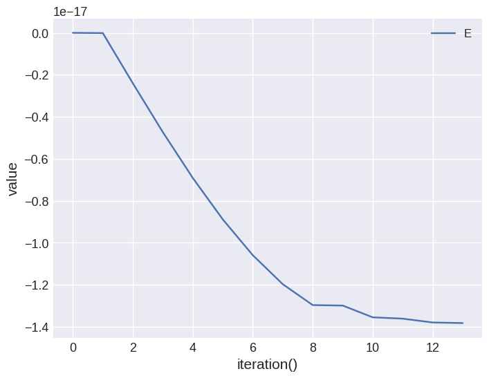
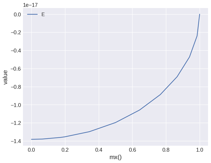
By fecault, iteration is showed on the \(x\)-axis. We can change that by passing x variable. For example:
[5]:
system.table.mpl(x="mx", y=["E"])
micromagneticdata analysis#
Similar to all other drivers, we can use micromagneticdata package to analyse the data. We start by creationg the data object:
[6]:
import micromagneticdata as md

data = md.Data(name=system.name)
We can have a look at all drives we did so far:
[7]:
data.info
[7]:
| drive_number | date | time | driver | t | n | n_threads | adapter | start_time | adapter_version | output_step | end_time | elapsed_time | success | |
|---|---|---|---|---|---|---|---|---|---|---|---|---|---|---|
| 0 | 0 | 2023-01-16 | 17:35:54 | MinDriver | NaN | NaN | NaN | NaN | NaN | NaN | NaN | NaN | NaN | NaN |
| 1 | 1 | 2023-01-16 | 17:35:58 | TimeDriver | 2.000000e-09 | 200.0 | 4.0 | NaN | NaN | NaN | NaN | NaN | NaN | NaN |
| 2 | 2 | 2023-01-16 | 17:37:00 | MinDriver | NaN | NaN | NaN | NaN | NaN | NaN | NaN | NaN | NaN | NaN |
| 3 | 3 | 2023-01-16 | 17:37:04 | TimeDriver | 2.000000e-09 | 200.0 | 4.0 | NaN | NaN | NaN | NaN | NaN | NaN | NaN |
| 4 | 4 | 2023-01-16 | 17:37:28 | MinDriver | NaN | NaN | NaN | NaN | NaN | NaN | NaN | NaN | NaN | NaN |
| 5 | 5 | 2023-01-16 | 17:38:02 | MinDriver | NaN | NaN | NaN | NaN | NaN | NaN | NaN | NaN | NaN | NaN |
| 6 | 6 | 2023-01-16 | 17:38:06 | TimeDriver | 2.000000e-09 | 200.0 | 4.0 | NaN | NaN | NaN | NaN | NaN | NaN | NaN |
| 7 | 7 | 2023-10-10 | 16:55:09 | MinDriver | NaN | NaN | NaN | NaN | NaN | NaN | NaN | NaN | NaN | NaN |
| 8 | 8 | 2023-10-10 | 16:55:13 | TimeDriver | 2.000000e-09 | 200.0 | 4.0 | NaN | NaN | NaN | NaN | NaN | NaN | NaN |
| 9 | 9 | 2023-10-18 | 12:37:23 | MinDriver | NaN | NaN | NaN | NaN | NaN | NaN | NaN | NaN | NaN | NaN |
| 10 | 10 | 2023-10-18 | 12:39:38 | MinDriver | NaN | NaN | NaN | NaN | NaN | NaN | NaN | NaN | NaN | NaN |
| 11 | 11 | 2023-10-18 | 12:39:56 | TimeDriver | 2.000000e-09 | 200.0 | 4.0 | NaN | NaN | NaN | NaN | NaN | NaN | NaN |
| 12 | 12 | 2024-07-14 | 16:10:32 | MinDriver | NaN | NaN | NaN | oommfc | NaN | NaN | NaN | NaN | NaN | NaN |
| 13 | 13 | 2024-07-14 | 16:10:37 | TimeDriver | 2.000000e-09 | 200.0 | 4.0 | oommfc | NaN | NaN | NaN | NaN | NaN | NaN |
| 14 | 14 | 2025-02-02 | 14:11:40 | MinDriver | NaN | NaN | NaN | oommfc | 2025-02-02T14:11:40 | 0.64.1 | True | 2025-02-02T14:11:41 | 00:00:01 | True |
| 15 | 15 | 2025-02-02 | 14:11:46 | TimeDriver | 2.000000e-09 | 200.0 | 4.0 | oommfc | 2025-02-02T14:11:46 | 0.64.1 | NaN | NaN | NaN | NaN |
| 16 | 16 | 2025-02-02 | 14:14:09 | MinDriver | NaN | NaN | NaN | oommfc | 2025-02-02T14:14:09 | 0.64.1 | True | 2025-02-02T14:14:10 | 00:00:01 | True |
| 17 | 17 | 2025-02-02 | 14:14:14 | TimeDriver | 2.000000e-09 | 200.0 | 4.0 | oommfc | 2025-02-02T14:14:14 | 0.64.1 | NaN | 2025-02-02T14:14:15 | 00:00:02 | True |
| 18 | 18 | 2025-02-02 | 14:32:10 | MinDriver | NaN | NaN | NaN | oommfc | 2025-02-02T14:32:10 | 0.65.0 | True | 2025-02-02T14:32:11 | 00:00:01 | True |
There is only one drive and we can get it by passing 0 (ot -1) as an index:
[8]:
drive = data[0]
We can now plot the magnetisation at individual iterations, by indexing it again with the step number and do all usual operations allowed by discretisedfield.Field object.
[9]:
drive[0]
[9]:
- Mesh
- Region
- pmin = [-5e-08, -5e-08, 0.0]
- pmax = [5e-08, 5e-08, 1e-08]
- dims = ['x', 'y', 'z']
- units = ['m', 'm', 'm']
- n = [20, 20, 2]
- Region
- nvdim = 3
- vdims:
- x
- y
- z
- unit = A/m
The number of steps in the drive is:
[10]:
drive.n
[10]:
14
Let us now create an interactive plot. For details on how to create custom interactive plots, please have a look at other tutorials.
[11]:
drive.register_callback(lambda f: f.sel("y")).hv(kdims=["x", "z"]).opts(frame_width=800)
[11]: