Tutorial 04: Dzyaloshinskii-Moriya energy term

Dzyaloshinskii-Moriya energy density, depending on the crystallographic class, is computed as

\[\begin{split}\mathbf{w_\text{dmi}} = \left\{ \begin{array}{ll} D \mathbf{m} \cdot (\nabla \times \mathbf{m}), & \text{for}\,\,T(O) \\ D ( \mathbf{m} \cdot \nabla m_{z} - m_{z} \nabla \cdot \mathbf{m}), & \text{for}\,\,C_{nv} \\ D\mathbf{m} \cdot \left( \frac{\partial \mathbf{m}}{\partial x} \times \hat{x} - \frac{\partial \mathbf{m}}{\partial y} \times \hat{y} \right), & \text{for}\,\,D_{2d} \\ \end{array} \right.\end{split}\]

where \(\mathbf{m}\) is the normalised (\(|\mathbf{m}|=1\)) magnetisation, and \(D\) is the DM energy constant. DMI energy term tends to align neighbouring magnetic moments perpendicular to each other.

In oommfc, \(\mathbf{m}\) is a part of the magnetisation field system.m. Therefore, only DMI energy constant \(D\) should be provided as an input parameter to uniquely define the Exchange energy term. \(D\) can be constant in space or spatially varying.

Spatially constant \(D\)

Let us start by assembling a simple simple simulation where \(D\) does not vary in space. The sample is a “one-dimensional” chain of magnetic moments. We are going to choose \(C_{nv}\) as the crystallographic class.

import discretisedfield as df
import micromagneticmodel as mm

import oommfc as oc

p1 = (-10e-9, 0, 0)
p2 = (10e-9, 1e-9, 1e-9)
cell = (1e-9, 1e-9, 1e-9)
region = df.Region(p1=p1, p2=p2)
mesh = df.Mesh(region=region, cell=cell)

The mesh is

mesh.k3d()

The system has a Hamiltonian, which consists of only DMI energy term.

D = 1e-3  # Dzyaloshinksii-Moriya energy constant (J/m**2)
system = mm.System(name="dmi_constant_D")
system.energy = mm.DMI(D=D, crystalclass="Cnv_z")

We are going to minimise the system’s energy using oommfc.MinDriver later. Therefore, we do not have to define the system’s dynamics equation. Finally, we need to define the system’s magnetisation (system.m). We are going to make it random with \(M_\text{s}=8\times10^{5} \,\text{Am}^{-1}\)

import random

import discretisedfield as df

Ms = 8e5  # saturation magnetisation (A/m)


def m_fun(pos):
    """Return random 3d vectors for initial random magnetisation"""
    return [2 * random.random() - 1, 2 * random.random() - 1, 2 * random.random() - 1]


system.m = df.Field(mesh, nvdim=3, value=m_fun, norm=Ms)

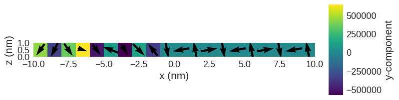
The magnetisation, we have set as initial values looks like:

system.m.k3d.vector(color_field=system.m.z)  # k3d plot

system.m.sel("y").mpl()  # matplotlib plot

Now, we can minimise the system’s energy by using oommfc.MinDriver.

md = oc.MinDriver()
md.drive(system)

Running OOMMF (ExeOOMMFRunner)[2023/10/18 12:35]... (0.4 s)

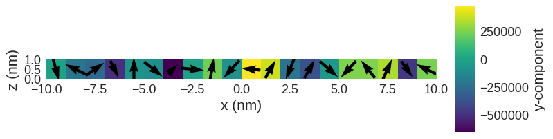
We expect that now all magnetic moments are aligned orthogonally to each other.

system.m.k3d.vector(color_field=system.m.z)  # k3d plot

system.m.sel("y").mpl()  # matplotlib plot

Spatially varying \(D\)

In the case of DMI, there is only one way how a parameter can be made spatially varying - using a dictionary.

In order to define a parameter using a dictionary, regions must be defined in the mesh. Regions are defined as a dictionary, whose keys are the strings and values are discretisedfield.Region objects, which take two corner points of the region as input parameters.

p1 = (-10e-9, 0, 0)
p2 = (10e-9, 1e-9, 1e-9)
cell = (1e-9, 1e-9, 1e-9)
subregions = {
    "region1": df.Region(p1=(-10e-9, 0, 0), p2=(0, 1e-9, 1e-9)),
    "region2": df.Region(p1=(0, 0, 0), p2=(10e-9, 1e-9, 1e-9)),
}
region = df.Region(p1=p1, p2=p2)
mesh = df.Mesh(region=region, cell=cell, subregions=subregions)

The regions we have defined are:

mesh.k3d.subregions()

Let us say there is no DMI energy (\(D=0\)) in region 1, whereas in region 2 \(D=10^{-3} \,\text{Jm}^{-2}\). Unlike Zeeman and anisotropy energy terms, the DMI energy constant is defined between cells. Therefore, it is necessary to also define the value of \(D\) between the two regions. This is achieved by adding another item to the dictionary with key 'region1:region2'. The object D is now defined as a dictionary:

D = {"region1": 0, "region2": 1e-3, "region1:region2": 0.5e-3}

The system object is

system = mm.System(name="dmi_dict_D")
system.energy = mm.DMI(D=D, crystalclass="Cnv_z")
system.m = df.Field(mesh, nvdim=3, value=m_fun, norm=Ms)

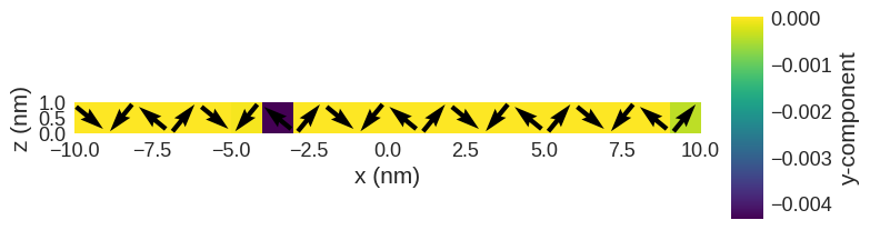
Its initial (and random) magnetisation is

system.m.k3d.vector(color_field=system.m.z)
system.m.sel("y").mpl()

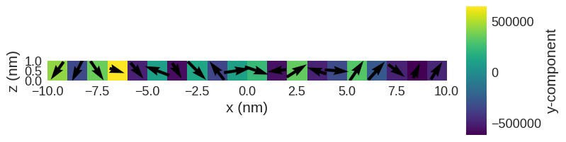
After we minimise the energy

md.drive(system)

Running OOMMF (ExeOOMMFRunner)[2023/10/18 12:35]... (0.2 s)

The magnetisation is as we expected. The magnetisation remains random in region 1, and it is orthogonally aligned in region 2.

system.m.k3d.vector(color_field=system.m.z)
system.m.sel("y").mpl()