
Line object#
In this tutorial, we show the basics of the line object. We start from the following field:
[1]:
import discretisedfield as df

mesh = df.Mesh(
    p1=(-10e-9, -10e-9, -10e-9), p2=(15e-9, 10e-9, 5e-9), cell=(1e-9, 1e-9, 1e-9)
)


def value_fun(point):
    x, y, z = point
    c = 1e9
    return (x * c, 2 * y * c, 3 * z * c)


field = df.Field(mesh, nvdim=3, value=value_fun, norm=1e6)
We create a line object by passing two points between which the line spans as well as the number of points we want to sample on that line:
[2]:
line = field.line(p1=(-10e-9, 0, 0), p2=(15e-9, 0, 0), n=25)
We can ask for the data on the line:
[3]:
line.data
[3]:
| r | x | y | z | vx | vy | vz | |
|---|---|---|---|---|---|---|---|
| 0 | 0.000000e+00 | -1.000000e-08 | 0.0 | 0.0 | -982466.610991 | 103417.537999 | 155126.306999 |
| 1 | 1.041667e-09 | -8.958333e-09 | 0.0 | 0.0 | -978240.074002 | 115087.067530 | 172630.601295 |
| 2 | 2.083333e-09 | -7.916667e-09 | 0.0 | 0.0 | -972305.585328 | 129640.744710 | 194461.117066 |
| 3 | 3.125000e-09 | -6.875000e-09 | 0.0 | 0.0 | -963624.111659 | 148249.863332 | 222374.794998 |
| 4 | 4.166667e-09 | -5.833333e-09 | 0.0 | 0.0 | -950255.268139 | 172773.685116 | 259160.527674 |
| 5 | 5.208333e-09 | -4.791667e-09 | 0.0 | 0.0 | -928279.121633 | 206284.249252 | 309426.373878 |
| 6 | 6.250000e-09 | -3.750000e-09 | 0.0 | 0.0 | -889000.889001 | 254000.254000 | 381000.381001 |
| 7 | 7.291667e-09 | -2.708333e-09 | 0.0 | 0.0 | -811107.105654 | 324442.842262 | 486664.263392 |
| 8 | 8.333333e-09 | -1.666667e-09 | 0.0 | 0.0 | -639602.149067 | 426401.432711 | 639602.149067 |
| 9 | 9.375000e-09 | -6.250000e-10 | 0.0 | 0.0 | -267261.241912 | 534522.483825 | 801783.725737 |
| 10 | 1.041667e-08 | 4.166667e-10 | 0.0 | 0.0 | 267261.241912 | 534522.483825 | 801783.725737 |
| 11 | 1.145833e-08 | 1.458333e-09 | 0.0 | 0.0 | 639602.149067 | 426401.432711 | 639602.149067 |
| 12 | 1.250000e-08 | 2.500000e-09 | 0.0 | 0.0 | 811107.105654 | 324442.842262 | 486664.263392 |
| 13 | 1.354167e-08 | 3.541667e-09 | 0.0 | 0.0 | 889000.889001 | 254000.254000 | 381000.381001 |
| 14 | 1.458333e-08 | 4.583333e-09 | 0.0 | 0.0 | 928279.121633 | 206284.249252 | 309426.373878 |
| 15 | 1.562500e-08 | 5.625000e-09 | 0.0 | 0.0 | 950255.268139 | 172773.685116 | 259160.527674 |
| 16 | 1.666667e-08 | 6.666667e-09 | 0.0 | 0.0 | 963624.111659 | 148249.863332 | 222374.794998 |
| 17 | 1.770833e-08 | 7.708333e-09 | 0.0 | 0.0 | 972305.585328 | 129640.744710 | 194461.117066 |
| 18 | 1.875000e-08 | 8.750000e-09 | 0.0 | 0.0 | 978240.074002 | 115087.067530 | 172630.601295 |
| 19 | 1.979167e-08 | 9.791667e-09 | 0.0 | 0.0 | 982466.610991 | 103417.537999 | 155126.306999 |
| 20 | 2.083333e-08 | 1.083333e-08 | 0.0 | 0.0 | 985578.834374 | 93864.650893 | 140796.976339 |
| 21 | 2.187500e-08 | 1.187500e-08 | 0.0 | 0.0 | 987934.593051 | 85907.355918 | 128861.033876 |
| 22 | 2.291667e-08 | 1.291667e-08 | 0.0 | 0.0 | 989759.478081 | 79180.758246 | 118771.137370 |
| 23 | 2.395833e-08 | 1.395833e-08 | 0.0 | 0.0 | 991201.182589 | 73422.309821 | 110133.464732 |
| 24 | 2.500000e-08 | 1.500000e-08 | 0.0 | 0.0 | 992359.570702 | 68438.591083 | 102657.886624 |
Dimension of the value:
[4]:
line.dim
[4]:
3
Length of the line:
[5]:
line.length
[5]:
2.5e-08
The number of points:
[6]:
line.n
[6]:
25
The columns storing coordinates of points are:
[7]:
line.point_columns
[7]:
['x', 'y', 'z']
Similarly, the columns storing field values are:
[8]:
line.value_columns
[8]:
['vx', 'vy', 'vz']
By default, value columns start with v, but we can rename them:
[9]:
line.value_columns = ["xval", "yval", "zval"]
Line data is now:
[10]:
line.data
[10]:
| r | x | y | z | xval | yval | zval | |
|---|---|---|---|---|---|---|---|
| 0 | 0.000000e+00 | -1.000000e-08 | 0.0 | 0.0 | -982466.610991 | 103417.537999 | 155126.306999 |
| 1 | 1.041667e-09 | -8.958333e-09 | 0.0 | 0.0 | -978240.074002 | 115087.067530 | 172630.601295 |
| 2 | 2.083333e-09 | -7.916667e-09 | 0.0 | 0.0 | -972305.585328 | 129640.744710 | 194461.117066 |
| 3 | 3.125000e-09 | -6.875000e-09 | 0.0 | 0.0 | -963624.111659 | 148249.863332 | 222374.794998 |
| 4 | 4.166667e-09 | -5.833333e-09 | 0.0 | 0.0 | -950255.268139 | 172773.685116 | 259160.527674 |
| 5 | 5.208333e-09 | -4.791667e-09 | 0.0 | 0.0 | -928279.121633 | 206284.249252 | 309426.373878 |
| 6 | 6.250000e-09 | -3.750000e-09 | 0.0 | 0.0 | -889000.889001 | 254000.254000 | 381000.381001 |
| 7 | 7.291667e-09 | -2.708333e-09 | 0.0 | 0.0 | -811107.105654 | 324442.842262 | 486664.263392 |
| 8 | 8.333333e-09 | -1.666667e-09 | 0.0 | 0.0 | -639602.149067 | 426401.432711 | 639602.149067 |
| 9 | 9.375000e-09 | -6.250000e-10 | 0.0 | 0.0 | -267261.241912 | 534522.483825 | 801783.725737 |
| 10 | 1.041667e-08 | 4.166667e-10 | 0.0 | 0.0 | 267261.241912 | 534522.483825 | 801783.725737 |
| 11 | 1.145833e-08 | 1.458333e-09 | 0.0 | 0.0 | 639602.149067 | 426401.432711 | 639602.149067 |
| 12 | 1.250000e-08 | 2.500000e-09 | 0.0 | 0.0 | 811107.105654 | 324442.842262 | 486664.263392 |
| 13 | 1.354167e-08 | 3.541667e-09 | 0.0 | 0.0 | 889000.889001 | 254000.254000 | 381000.381001 |
| 14 | 1.458333e-08 | 4.583333e-09 | 0.0 | 0.0 | 928279.121633 | 206284.249252 | 309426.373878 |
| 15 | 1.562500e-08 | 5.625000e-09 | 0.0 | 0.0 | 950255.268139 | 172773.685116 | 259160.527674 |
| 16 | 1.666667e-08 | 6.666667e-09 | 0.0 | 0.0 | 963624.111659 | 148249.863332 | 222374.794998 |
| 17 | 1.770833e-08 | 7.708333e-09 | 0.0 | 0.0 | 972305.585328 | 129640.744710 | 194461.117066 |
| 18 | 1.875000e-08 | 8.750000e-09 | 0.0 | 0.0 | 978240.074002 | 115087.067530 | 172630.601295 |
| 19 | 1.979167e-08 | 9.791667e-09 | 0.0 | 0.0 | 982466.610991 | 103417.537999 | 155126.306999 |
| 20 | 2.083333e-08 | 1.083333e-08 | 0.0 | 0.0 | 985578.834374 | 93864.650893 | 140796.976339 |
| 21 | 2.187500e-08 | 1.187500e-08 | 0.0 | 0.0 | 987934.593051 | 85907.355918 | 128861.033876 |
| 22 | 2.291667e-08 | 1.291667e-08 | 0.0 | 0.0 | 989759.478081 | 79180.758246 | 118771.137370 |
| 23 | 2.395833e-08 | 1.395833e-08 | 0.0 | 0.0 | 991201.182589 | 73422.309821 | 110133.464732 |
| 24 | 2.500000e-08 | 1.500000e-08 | 0.0 | 0.0 | 992359.570702 | 68438.591083 | 102657.886624 |
Line visualisation#
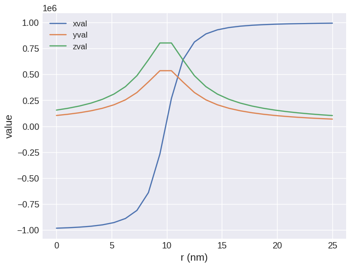
Default plot is:
[11]:
line.mpl()
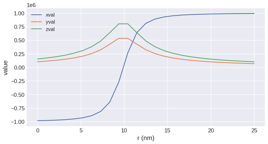
We can change the size of the plot:
[12]:
line.mpl(figsize=(10, 5))
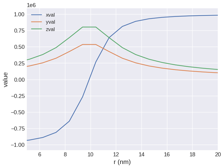
Also, we can limit the values on the x-axis:
[13]:
line.mpl(xlim=[5e-9, 20e-9])
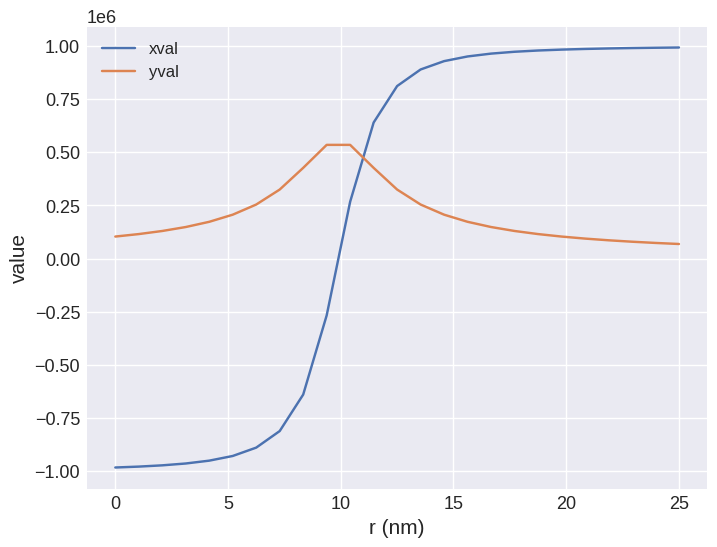
and we can choose what we want to plot:
[14]:
line.mpl(yaxis=["xval", "yval"])
Similar to all other plots, we can build interactive plots:
[15]:
@df.interact(xlim=line.slider(continuous_update=False), yaxis=line.selector())
def myplot(xlim, yaxis):
    return line.mpl(figsize=(10, 6), yaxis=yaxis, marker="o", xlim=xlim)