Table interactive plot

In previous tutorials we showed how to plot the data as well as some widgets which are a part of the table object. In this tutorial, we show how an interactive plot can be built.

Let us demonstrate plotting using the data from an example file:

import os

import ubermagtable as ut

# Sample OOMMF .odt file
dirname = os.path.join("..", "ubermagtable", "tests", "test_sample")
odtfile = os.path.join(dirname, "oommf-old-file2.odt")

table = ut.Table.fromfile(odtfile, x="t")

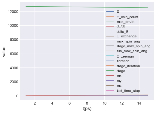
By calling mpl method, default plot is shown:

table.mpl()

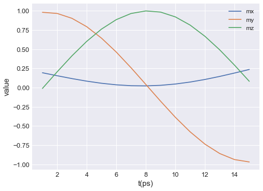
By default, all data columns are plotted. To select only certain data columns, y can be passed. y is a list of strings, where each string matches one of the columns. For instance, if we want to plot the average magnetisation components, the plot is:

table.mpl(y=["mx", "my", "mz"])

Now, let us say we want to interactively choose data columns we want to plot on y-axis of the plot. We start by putting our plotting inside a function and exposing the argument we want to choose:

def my_interactive_plot(y):
    table.mpl(y=y)

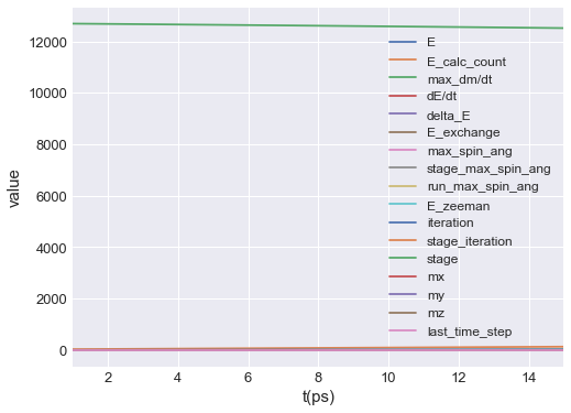
Having the function defined, we have to call it with required yaxis argument in order to get the plot. For example,

my_interactive_plot(y=["mx", "my", "mz"])

To interactively change the values of yaxis, we have to:

1. decorate the function using ubermagtable.interact and

2. assign a widget to the yaxis in the ubermagtable.interact argument list.

# NBVAL_IGNORE_OUTPUT
@ut.interact(y=table.selector())
def my_interactive_plot(y):
    table.mpl(y=y)

The plot, together with a selector widget is shown. In order to select multiple data columns from the widget list, we hold Ctrl (Windows, Linux) or Cmd (MacOS) and select multiple data columns.

Another argument of the plot we can interact with is the range of time values on the horizontal axis. For that, we have to expose xlim and assign it a slider widget.

# NBVAL_IGNORE_OUTPUT
@ut.interact(y=table.selector(), xlim=table.slider())
def my_interactive_plot(y, xlim):
    table.mpl(y=y, xlim=xlim)

This way, by exposing the axes and passing any allowed matplotlib.pyplot.plot argument, we can customise the plot any way we like (as long as it is allowed by matplotlib).