
[1]:
import holoviews as hv

hv.extension("bokeh", logo=False)
hv.output(widget_location="bottom")
Interactive plots#
This notebook show how to use Holoviews based plotting methods to create interactive plots of the magnetisation or derived quantities. The interface is the same as in discretisedfield.Field.hv. For details on the different plotting methods refer to the documentation of Holoviews based plotting in discretisedfield.
[2]:
import os

import discretisedfield.tools as dft
import numpy as np

import micromagneticdata as md
We have a set of example simulations stored in the test directory of micromagneticdata that we use to demonstrate its functionality.
[3]:
dirname = os.path.join("..", "micromagneticdata", "tests", "test_sample")
Visualising computed magnetisation data#
First, we creata a Data object. We need to pass the name of the micromagneticmodel.System that we used to run the simulation and optionally an additional path to the base directory.
[4]:
data = md.Data(name="rectangle", dirname=dirname)
The Data object contains all simulation runs of the System. These are called drives.
[5]:
data.info
[5]:
| drive_number | date | time | start_time | adapter | adapter_version | driver | t | n | end_time | elapsed_time | success | info.json | output_step | |
|---|---|---|---|---|---|---|---|---|---|---|---|---|---|---|
| 0 | 0 | 2025-05-31 | 22:02:42 | 2025-05-31T22:02:42 | oommfc | 0.65.0 | TimeDriver | 0.0 | 25 | 2025-05-31T22:02:42 | 00:00:01 | True | available | <NA> |
| 1 | 1 | 2025-05-31 | 22:02:42 | 2025-05-31T22:02:42 | mumax3c | 0.3.0 | TimeDriver | 0.0 | 15 | 2025-05-31T22:02:42 | 00:00:01 | True | available | <NA> |
| 2 | 2 | 2025-05-31 | 22:02:42 | 2025-05-31T22:02:42 | mumax3c | 0.3.0 | TimeDriver | 0.0 | 250 | 2025-05-31T22:02:43 | 00:00:01 | True | available | <NA> |
| 3 | 3 | 2025-05-31 | 22:02:43 | 2025-05-31T22:02:43 | mumax3c | 0.3.0 | RelaxDriver | <NA> | <NA> | 2025-05-31T22:02:43 | 00:00:01 | True | available | <NA> |
| 4 | 4 | 2025-05-31 | 22:02:43 | 2025-05-31T22:02:43 | mumax3c | 0.3.0 | MinDriver | <NA> | <NA> | 2025-05-31T22:02:43 | 00:00:01 | True | available | <NA> |
| 5 | 5 | 2025-05-31 | 22:02:43 | 2025-05-31T22:02:43 | oommfc | 0.65.0 | TimeDriver | 0.0 | 5 | 2025-05-31T22:02:44 | 00:00:01 | True | available | <NA> |
| 6 | 6 | 2025-05-31 | 22:02:44 | 2025-05-31T22:02:44 | oommfc | 0.65.0 | MinDriver | <NA> | <NA> | 2025-05-31T22:02:44 | 00:00:01 | True | available | True |
Time evolution of the magnetisation#
[6]:
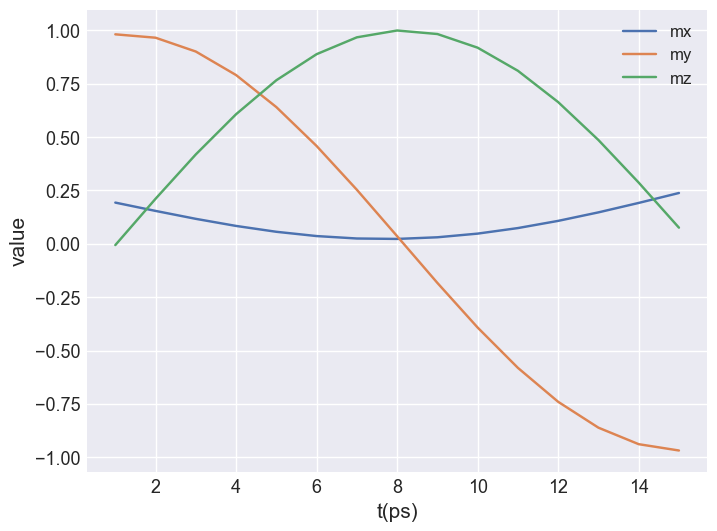
time_drive = data[1]
We first create a plot for the averaged magnetisation components to better understand the behaviour of the system. We can see a precession of all three components of the averaged magnetisation.
[7]:
time_drive.table.mpl(y=["mx", "my", "mz"])
We can use the .hv convenience method to create a plot similar to the plotting functionality in discretisedfield. We get an additional slider for the time variable.
We manually set the colorlimit to (-Ms, Ms) and use a different colormap.
[8]:
time_drive.hv(
    kdims=["x", "y"],
    scalar_kw={"clim": (-800000, 800000), "cmap": "coolwarm"},
)
[8]:
We can see that the magnetisation direction per time-step is uniform throughout the sample.
[9]:
time_drive.hv(
    kdims=["y", "z"],
    scalar_kw={"clim": (-800000, 800000), "cmap": "cividis"},
)
[9]:
Resampling can be done like in discretisedfield using a tuple (to only affect kdims)
[10]:
time_drive.hv(
    kdims=["x", "y"],
    scalar_kw={"clim": (-800000, 800000), "cmap": "coolwarm"},
    vector_kw={"n": (10, 6)},
)
[10]:
Combining multiple drives#
We can combine multiple consecutive time drives to get a single plot showing the whole simulation.
[11]:
full_time_drive = data[0] << data[1] << data[2]
Again, we first show the scalar plot to better understand the data.
[12]:
full_time_drive.table.mpl(y=["mx", "my", "mz"])
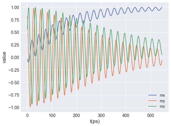
Now, we can create an interactive plot. Note that the resulution of the time slider changes as we “jump” from the first two drives with fine resolution to the last one with a coarser resolution.
[13]:
full_time_drive.hv(
    kdims=["x", "y"],
    scalar_kw={"clim": (-800000, 800000), "cmap": "coolwarm"},
    vector_kw={"n": (10, 5)},
)
[13]:
Computing derived quantities#
In this section we look at a different example simulation, the dynamics of a magnetic vortex. We demonstrate how to compute derived quantities based on a series of magnetisation samples from the time drive.
[14]:
data = md.Data(name="vortex_dynamics", dirname=dirname)
[15]:
data.info
[15]:
| drive_number | date | time | start_time | adapter | adapter_version | driver | end_time | elapsed_time | success | info.json | t | n | |
|---|---|---|---|---|---|---|---|---|---|---|---|---|---|
| 0 | 0 | 2025-05-31 | 22:02:44 | 2025-05-31T22:02:44 | oommfc | 0.65.0 | MinDriver | 2025-05-31T22:02:44 | 00:00:01 | True | available | <NA> | <NA> |
| 1 | 1 | 2025-05-31 | 22:02:44 | 2025-05-31T22:02:44 | oommfc | 0.65.0 | MinDriver | 2025-05-31T22:02:44 | 00:00:01 | True | available | <NA> | <NA> |
| 2 | 2 | 2025-05-31 | 22:02:44 | 2025-05-31T22:02:44 | oommfc | 0.65.0 | TimeDriver | 2025-05-31T22:02:46 | 00:00:03 | True | available | 0.0 | 250 |
Time evolution of the magnetisation#
[16]:
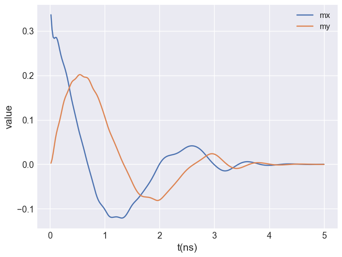
time_drive = data[2]
We first create a plot for the averaged magnetisation components to better understand the behaviour of the system. We can see a damped precession in x and y.
[17]:
time_drive.table.mpl(y=["mx", "my"])
We can also create an interactive plot for the full magnetisation.
[18]:
time_drive.hv(kdims=["x", "y"])
[18]:
Selecting only a part of the drive#
We can use slicing notation to select and plot only a part of the data. Here, we select the every 5th of the first 100 samples.
[19]:
time_drive[:100:5].hv(kdims=["x", "y"])
[19]:
Normalised magnetisation#
To plot the normalised field, we can register a callback function. This function will be applied to each field in the drive before the field is passed to the plotting method. The input argument to this function is a discretisedfield.Field. Here, we have a simple function that computes the normalised field (field.orientation). As the code for this function is very short, we can use a lambda function and define it directly inside the register_callback method. The
register_callback method returns a new drive object that we can plot.
If you are not familiar with lambda functions you can also use normal functions as demonstrated in one of the next examples.
[20]:
time_drive.register_callback(lambda field: field.orientation).hv(kdims=["x", "y"])
[20]:
Topological charge density - example 1#
To give a second example, we compute the topological charge density in the xy plane. This operation is implemented in discretisedfield.tools. However, discretisedfield.tools.topological_charge_density can only work on a single plane. Therefore, we first select one plane in the z direction and afterwards compute the topological charge density.
Here, we first create a new object and afterwards plot it.
[21]:
time_drive_tcd_1 = time_drive.register_callback(
    lambda field: dft.topological_charge_density(field.sel("z"))
)
[22]:
time_drive_tcd_1.hv.scalar(kdims=["x", "y"], cmap="plasma")
[22]:
Topological charge density - example 2#
If multiple callbacks are registered, these will be applied one after another in the order that they have been registered. Do demonstrate this, we repeat the example of the topological charge density in two steps:
We select a xy single plane
We compute the topological charge density on that plane
Furthermore, we define our functions outside the register_callback method in this example.
[23]:
def select_plane(field):
    return field.sel("z")


def topological_charge_density(field):
    return dft.topological_charge_density(field)


time_drive_tcd_2 = time_drive.register_callback(select_plane)
time_drive_tcd_2 = time_drive_tcd_2.register_callback(topological_charge_density)
time_drive_tcd_2.hv.scalar(kdims=["x", "y"], cmap="plasma")
[23]:
It is possible to display all callbacks, as follows. Note however, that this information is difficult to read when using lambda funtions as their names are not very explanatory.
[24]:
time_drive_tcd_2.callbacks
[24]:
[<function __main__.select_plane(field)>,
 <function __main__.topological_charge_density(field)>]
Hysteresis simulation#
TODO
[25]:
data = md.Data(name="hysteresis", dirname=dirname)
[26]:
data.info
[26]:
| drive_number | date | time | start_time | adapter | adapter_version | driver | Hmin | Hmax | n | end_time | elapsed_time | success | info.json | |
|---|---|---|---|---|---|---|---|---|---|---|---|---|---|---|
| 0 | 0 | 2025-05-31 | 22:02:46 | 2025-05-31T22:02:46 | oommfc | 0.65.0 | HysteresisDriver | [0, 0, -795774.7154594767] | [0, 0, 795774.7154594767] | 21 | 2025-05-31T22:02:47 | 00:00:01 | True | available |
Time evolution of the magnetisation#
[27]:
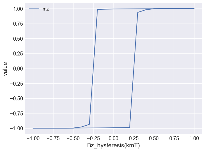
drive = data[0]
We first create a plot for the averaged magnetisation components to better understand the behaviour of the system. We can see a damped precession in x and y.
[28]:
drive.table.mpl(x="Bz_hysteresis", y=["mz"])
We can also create an interactive plot for the full magnetisation.
Note: we have to change the independent variable drive.x to the iteration (stage) to be able to see the full loop. The default value (B_hysteresis) is not unique.
[29]:
drive.x = "stage"
[30]:
Ms = np.max(np.abs(drive.m0.norm.array))

drive.register_callback(lambda field: field.z).hv(
    kdims=["x", "z"], scalar_kw={"clim": (-Ms, Ms)}
)
[30]: