Time-varying field

In this tutorial, we introduce how a time-dependent external magnetic field can be defined in energy equation. We start by importing the modules we are going to use:

import oommfc as mc
import discretisedfield as df
import micromagneticmodel as mm

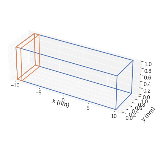
For the sample, we choose a one-dimensional chain of magnetic moments.

p1 = (-10e-9, 0, 0)
p2 = (10e-9, 1e-9, 1e-9)
cell = (1e-9, 1e-9, 1e-9)
region = df.Region(p1=p1, p2=p2)
mesh = df.Mesh(region=region, cell=cell)

The mesh is:

mesh.mpl(box_aspect=(10, 3, 3))

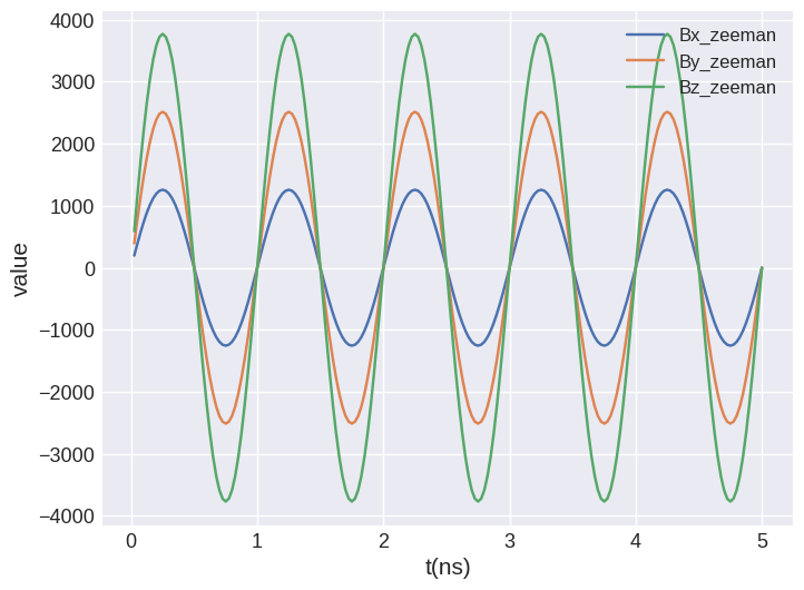
Now, we can define the system object and add a time-dependent sine-wave field to our energy equation. We need to pass:

• Field H which is multiplied by time-dependent function at each time step,

• wave shape func='sin'

• frequency f, and

• time shift t0.

Accordingly, the time-dependent Zeeman field is then:

\[\mathbf{H}(t) = \mathbf{H}_\text{amp}\sin(2\pi f (t-t_{0}))\]

system = mm.System(name='time_dependent_field')

system.energy = mm.Exchange(A=1.6e-11) + mm.Zeeman(H=(1e6, 2e6, 3e6), func='sin', f=1e9, t0=1e-9)
system.dynamics = mm.Precession(gamma0=mm.consts.gamma0) + mm.Damping(alpha=1e-5)

system.m = df.Field(mesh, nvdim=3, value=(0, 0, 1), norm=1.1e6)

Now, we can run the simulation using TimeDriver:

td = mc.TimeDriver()
td.drive(system, t=5e-9, n=200)

Running OOMMF (ExeOOMMFRunner)[2023/10/23 16:03]... (2.3 s)

In the system table, there are columns with field values:

system.table.data

	E	E_calc_count	max_dm/dt	dE/dt	delta_E	E_exchange	max_spin_ang_exchange	stage_max_spin_ang_exchange	run_max_spin_ang_exchange	E_zeeman	...	By_zeeman	Bz_zeeman	iteration	stage_iteration	stage	mx	my	mz	last_time_step	t
0	-1.297563e-20	25.0	4.434031e+03	-5.147568e-10	-1.812700e-21	0.0	0.0	0.0	0.0	-1.297563e-20	...	3.931627e+02	5.897440e+02	3.0	3.0	0.0	0.758989	0.183653	0.624666	3.515634e-12	2.500000e-11
1	-2.562001e-20	56.0	8.766104e+03	-4.954602e-10	-1.204656e-21	0.0	0.0	0.0	0.0	-2.562001e-20	...	7.766444e+02	1.164967e+03	9.0	5.0	1.0	0.090633	-0.038564	0.995137	2.425770e-12	5.000000e-11
2	-3.759093e-20	105.0	1.290846e+04	-4.636140e-10	-1.221901e-21	0.0	0.0	0.0	0.0	-3.759093e-20	...	1.141003e+03	1.711504e+03	17.0	7.0	2.0	0.784284	0.261449	0.562622	2.631440e-12	7.500000e-11
3	-4.863542e-20	184.0	1.673341e+04	-4.207088e-10	-6.112468e-22	0.0	0.0	0.0	0.0	-4.863542e-20	...	1.477265e+03	2.215898e+03	30.0	12.0	3.0	0.015202	-0.010857	0.999825	1.449728e-12	1.000000e-10
4	-5.848036e-20	299.0	2.014752e+04	-3.675974e-10	-2.915541e-22	0.0	0.0	0.0	0.0	-5.848036e-20	...	1.777153e+03	2.665730e+03	48.0	17.0	4.0	0.497085	-0.051994	0.866143	7.913664e-13	1.250000e-10
...	...	...	...	...	...	...	...	...	...	...	...	...	...	...	...	...	...	...	...	...	...
195	4.436379e-20	20614.0	1.906705e+04	-3.837992e-10	-2.268306e-22	0.0	0.0	0.0	0.0	4.436379e-20	...	-1.477265e+03	-2.215898e+03	3450.0	15.0	195.0	-0.020176	-0.114665	0.993199	5.918021e-13	4.900000e-09
196	3.422674e-20	20687.0	1.474584e+04	-4.221479e-10	-5.046823e-22	0.0	0.0	0.0	0.0	3.422674e-20	...	-1.141003e+03	-1.711504e+03	3463.0	12.0	196.0	0.848044	0.209072	0.486939	1.197700e-12	4.925000e-09
197	2.328011e-20	20742.0	1.004530e+04	-4.502211e-10	-1.083878e-21	0.0	0.0	0.0	0.0	2.328011e-20	...	-7.766444e+02	-1.164967e+03	3473.0	9.0	197.0	0.063640	-0.149399	0.986727	2.412896e-12	4.950000e-09
198	1.178128e-20	20779.0	5.087140e+03	-4.673789e-10	-2.358762e-21	0.0	0.0	0.0	0.0	1.178128e-20	...	-3.931627e+02	-5.897440e+02	3480.0	6.0	198.0	0.822805	0.116178	0.556322	5.059389e-12	4.975000e-09
199	6.088592e-34	20804.0	2.629445e-10	-4.731610e-10	-2.217703e-21	0.0	0.0	0.0	0.0	6.088592e-34	...	-2.032019e-11	-3.048028e-11	3485.0	4.0	199.0	-0.041748	-0.107200	0.993361	4.687671e-12	5.000000e-09

200 rows × 22 columns

system.table.mpl(y=['Bx_zeeman', 'By_zeeman', 'Bz_zeeman'])

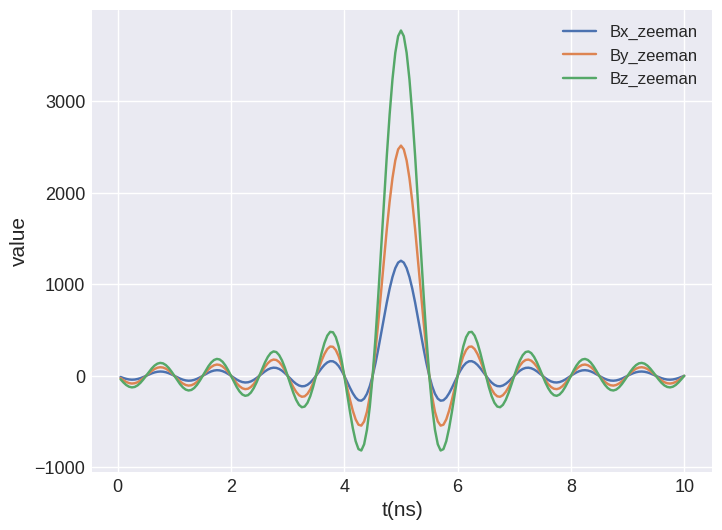
Similarly, we can define a cardinal sine wave (“sinc pulse”). We need to pass:

• Field H which is multiplied by time-dependent function at each time step,

• wave shape wave='sinc'

• cut-off frequency f, and

• time shift t0.

Accordingly, the time-dependent Zeeman field is then:

\[\mathbf{H}(t) = \mathbf{H}_\text{amp}\text{sinc}(2\pi f_{c} (t-t_{0})) = \mathbf{H}_\text{amp}\frac{\text{sinc}(2\pi f_{c} (t-t_{0}))}{2\pi f_{c} (t-t_{0})}\]

system = mm.System(name='time_dependent_field')

system.energy = (mm.Exchange(A=1.6e-11) +
                 mm.Zeeman(H=(1e6, 2e6, 3e6), func='sinc', f=1e9, t0=5e-9))
system.dynamics = mm.Precession(gamma0=mm.consts.gamma0) + mm.Damping(alpha=1e-5)

system.m = df.Field(mesh, nvdim=3, value=(0, 0, 1), norm=1.1e6)

td = mc.TimeDriver()
td.drive(system, t=10e-9, n=200)

system.table.mpl(y=['Bx_zeeman', 'By_zeeman', 'Bz_zeeman'])

Running OOMMF (ExeOOMMFRunner)[2023/10/23 16:03]... (1.3 s)