Spatially varying parameters 1#
In this tutorial, we explore different ways of defining a spatially varying parameter. As an example, we use the Zeeman energy term.
Spatially constant \(\mathbf{H}\)#
Let us start by assembling a simple simulation where \(\mathbf{H}\) does not vary in space. The sample is a “one-dimensional” chain of magnetic moments.
[1]:
import oommfc as mc
import discretisedfield as df
import micromagneticmodel as mm

p1 = (-10e-9, 0, 0)
p2 = (10e-9, 1e-9, 1e-9)
cell = (1e-9, 1e-9, 1e-9)
region = df.Region(p1=p1, p2=p2)
mesh = df.Mesh(region=region, cell=cell)
The system has an energy equation, which consists of only Zeeman energy term.
[2]:
H = (0, 0, 1e6)  # external magnetic field (A/m)
system = mm.System(name="zeeman_constant_H")
system.energy = mm.Zeeman(H=H)
We are going to minimise the system’s energy using oommfc.MinDriver later. Therefore, we do not have to define the system’s dynamics equation. Finally, we need to define the system’s magnetisation (system.m). We are going to make it random with \(M_\text{s}=8\times10^{5} \,\text{Am}^{-1}\)
[3]:
import random
import discretisedfield as df

Ms = 8e5  # saturation magnetisation (A/m)


def m_fun(pos):
    return [2 * random.random() - 1 for i in range(3)]


system.m = df.Field(mesh, nvdim=3, value=m_fun, norm=Ms)
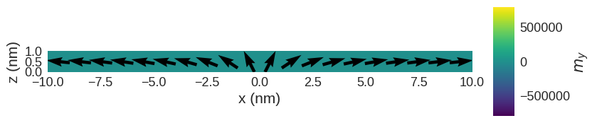
The magnetisation, we set is
[4]:
system.m.sel("y").mpl(
    scalar_kw={"colorbar_label": "$m_y$", "clim": (-Ms, Ms)}, figsize=(10, 2)
)
Now, we can minimise the system’s energy by using oommfc.MinDriver.
[5]:
md = mc.MinDriver()
md.drive(system)
Running OOMMF (ExeOOMMFRunner)[2023/10/23 16:07]... (0.3 s)
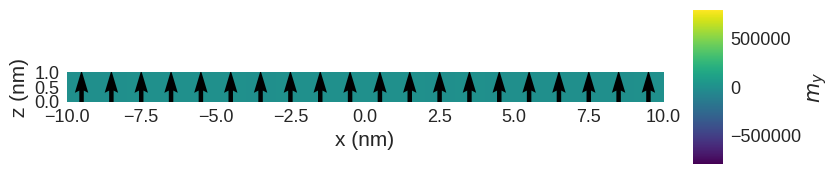
We expect that now all magnetic moments are aligned parallel to the external magnetic field (in the \(z\)-direction).
[6]:
system.m.sel("y").mpl(
    scalar_kw={"colorbar_label": "$m_y$", "clim": (-Ms, Ms)}, figsize=(10, 2)
)
Spatially varying H#
There are two different ways how a parameter can be made spatially varying, by using:
Dictionary
discretisedfield.Field
Dictionary
In order to define a parameter using a dictionary, subregions must be defined in the mesh. Subregions are defined as a dictionary, whose keys are the strings and values are discretisedfield.Region objects, which take two corner points of the region as input parameters.
[7]:
p1 = (-10e-9, 0, 0)
p2 = (10e-9, 1e-9, 1e-9)
cell = (1e-9, 1e-9, 1e-9)
subregions = {
    "subregion1": df.Region(p1=(-10e-9, 0, 0), p2=(0, 1e-9, 1e-9)),
    "subregion2": df.Region(p1=(0, 0, 0), p2=(10e-9, 1e-9, 1e-9)),
}

region = df.Region(p1=p1, p2=p2)
mesh = df.Mesh(region=region, cell=cell, subregions=subregions)
Let us say we want to apply the external magnetic field \(\mathbf{H}\) in region 1 in the \(x\)-direction and in region 2 in the negative \(z\)-direction. H is now defined as a dictionary:
[8]:
H = {"subregion1": (1e6, 0, 0), "subregion2": (0, 0, -1e6)}
The system object is
[9]:
system = mm.System(name="zeeman_dict_H")
system.energy = mm.Zeeman(H=H)
system.m = df.Field(mesh, nvdim=3, value=m_fun, norm=Ms)
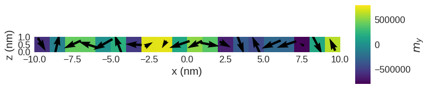
Its magnetisation is
[10]:
system.m.sel("y").mpl(
    scalar_kw={"colorbar_label": "$m_y$", "clim": (-Ms, Ms)}, figsize=(10, 2)
)
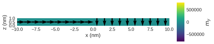
After we minimise the energy
[11]:
md.drive(system)
Running OOMMF (ExeOOMMFRunner)[2023/10/23 16:07]... (0.2 s)
The magnetisation is as we expected.
[12]:
system.m.sel("y").mpl(
    scalar_kw={"colorbar_label": "$m_y$", "clim": (-Ms, Ms)}, figsize=(10, 2)
)
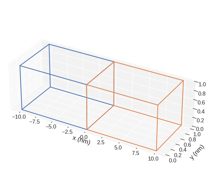
[13]:
mesh.mpl.subregions(box_aspect=(10, 3.5, 3), figsize=(8, 8))
``discretisedfield.Field``
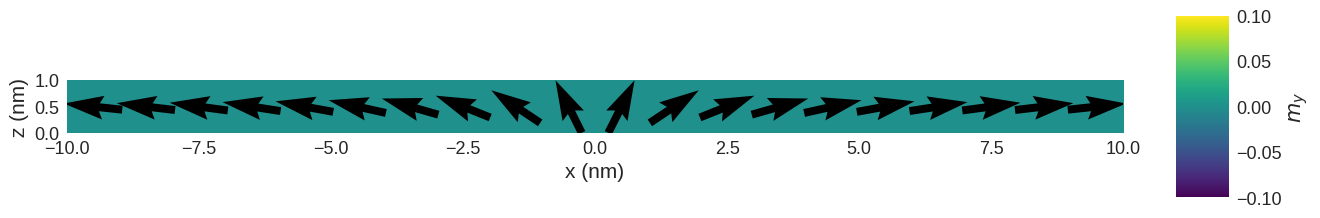
Let us say that the external magnetic field varies in space as
where \(c=10^{9}\) and the entire field is normalised with \(H = 10^{6} \,\text{Am}^{-1}\). The value of a spatially varying field is set using a Python function.
[14]:
def H_fun(point):
    x, y, z = point
    c = 1e9
    return (c * c * x, 0, c)
The external magnetic field is
[15]:
H = df.Field(mesh, nvdim=3, value=H_fun, norm=1e6)
H.sel("y").mpl(figsize=(15, 3), scalar_kw={"colorbar_label": "$m_y$"})
The system is
[16]:
system = mm.System(name="zeeman_field_H")
system.energy = mm.Zeeman(H=H)
system.m = df.Field(mesh, nvdim=3, value=m_fun, norm=Ms)
and its magnetisation is
[17]:
system.m.sel("y").mpl(
    scalar_kw={"colorbar_label": "$m_y$", "clim": (-Ms, Ms)}, figsize=(10, 2)
)
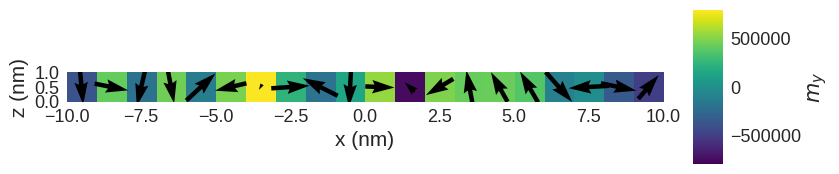
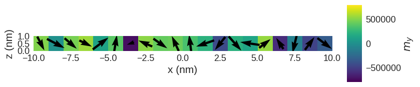
After the energy minimisation, the magnetisation is:
[18]:
md.drive(system)
system.m.sel("y").mpl(
    scalar_kw={"colorbar_label": "$m_y$", "clim": (-Ms, Ms)}, figsize=(10, 2)
)
Running OOMMF (ExeOOMMFRunner)[2023/10/23 16:07]... (0.2 s)