Analysing simulation results: Domain wall pair conversion#

Simulation#

Problem description#

We want to simulate a domain wall conversion in a two-dimensional thin film sample with:

exchange energy constant \(A = 15 \,\text{pJ}\,\text{m}^{-1}\),
Dzyaloshinskii-Moriya energy constant \(D = 3 \,\text{mJ}\,\text{m}^{-2}\),
uniaxial anisotropy constant \(K = 0.5 \,\text{MJ}\,\text{m}^{-3}\) with \(\hat{\mathbf{u}} = (0, 0, 1)\) in the out of plane direction,
gyrotropic ratio \(\gamma = 2.211 \times 10^{5} \,\text{m}\,\text{A}^{-1}\,\text{s}^{-1}\), and
Gilbert damping \(\alpha=0.3\).

Please carry out the following steps:

Create the following geometry with discretisation cell size \((2 \,\text{nm}, 2 \,\text{nm}, 2 \,\text{nm})\).
Initialise the magnetisation so that when relaxes, a domain pair is present in the narrower part of the geometry.
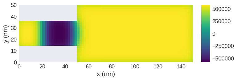
Relax the system. Is a domain wall pair contained in the constrained part?
Apply the spin polarised current in the positive \(x\) direction with velocity \(\mathbf{u} = (400, 0, 0) \,\text{m}\,\text{s}^{-1}\), with \(\beta=0.5\).
Evolve the system over \(0.2 \,\text{ns}\). What did you get? [1]

References#

[1] Zhou, Y., & Ezawa, M. (2014). A reversible conversion between a skyrmion and a domain-wall pair in a junction geometry. Nature Communications 5, 8. https://doi.org/10.1038/ncomms5652

Solution#

[1]:

import oommfc as oc
import discretisedfield as df
import micromagneticmodel as mm

Ms = 5.8e5  # saturation magnetisation (A/m)
A = 15e-12  # exchange energy constant (J/)
D = 3e-3  # Dzyaloshinkii-Moriya energy constant (J/m**2)
K = 0.5e6  # uniaxial anisotropy constant (J/m**3)
u = (0, 0, 1)  # easy axis
gamma0 = 2.211e5  # gyromagnetic ratio (m/As)
alpha = 0.3  # Gilbert damping

system = mm.System(name="dw_pair_conversion")
system.energy = (
    mm.Exchange(A=A)
    + mm.DMI(D=D, crystalclass="Cnv_z")
    + mm.UniaxialAnisotropy(K=K, u=u)
)
system.dynamics = mm.Precession(gamma0=2.211e5) + mm.Damping(alpha=alpha)

p1 = (0, 0, 0)
p2 = (150e-9, 50e-9, 2e-9)
cell = (2e-9, 2e-9, 2e-9)

region = df.Region(p1=p1, p2=p2)
mesh = df.Mesh(region=region, cell=cell)


def Ms_fun(pos):
    x, y, z = pos
    if x < 50e-9 and (y < 15e-9 or y > 35e-9):
        return 0
    else:
        return Ms


def m_init(pos):
    x, y, z = pos
    if 30e-9 < x < 40e-9:
        return (0.1, 0.1, -1)
    else:
        return (0.1, 0.1, 1)


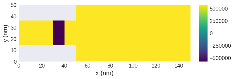
system.m = df.Field(mesh, nvdim=3, value=m_init, norm=Ms_fun, valid="norm")

system.m.z.sel("z").mpl.scalar()

../../_images/getting-started_notebooks_dw-pair-conversion_1_0.png

[2]:

md = oc.MinDriver()
md.drive(system)

system.m.z.sel("z").mpl.scalar()

Running OOMMF (ExeOOMMFRunner)[2024/08/09 18:15]... (0.8 s)

../../_images/getting-started_notebooks_dw-pair-conversion_2_1.png

[3]:

ux = 400  # velocity in x direction (m/s)
beta = 0.5  # non-adiabatic STT parameter

system.dynamics += mm.ZhangLi(u=ux, beta=beta)

[4]:

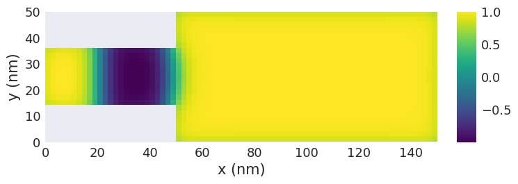
td = oc.TimeDriver()
td.drive(system, t=0.2e-9, n=200, verbose=2)

system.m.orientation.z.sel("z").mpl.scalar()

Running OOMMF (ExeOOMMFRunner)[2024/08/09 18:15] took 4.1 s

../../_images/getting-started_notebooks_dw-pair-conversion_4_2.png

As a result, we got a skyrmion formed in the wider region.

Data analysis#

We can use the micromagneticdata package for post processing of simulation data.

We get access to: - initial magnetisation - magnetisation snapshots from the simulation, e.g. at the timesteps specified in time_driver.drive(...) - tabular data recorded during the simulation via ubermagtable, e.g. total energy as a function of time

[5]:

import micromagneticdata as mdata

`Data`#

We can access data from past simulation runs based on the system name used to run the simulation.

[6]:

data = mdata.Data("dw_pair_conversion")

The Data object contains all simulation runs of the System, these are called drives. We can check how many drives does our data has:

[7]:

data.n

[7]:

We have used two drivers in our simulation, which has created two corresponding drives.

We can also extract the details using the info property.

[8]:

data.info

[8]:

	drive_number	date	time	driver	adapter	n_threads	t	n
0	0	2024-08-09	18:15:58	MinDriver	oommfc	None	NaN	NaN
1	1	2024-08-09	18:15:59	TimeDriver	oommfc	None	2.000000e-10	200.0

`Drive`#

We can explicitly check the two drivers seperately by indexing the Data object.

[9]:

data[0].info

[9]:

{'drive_number': 0,
 'date': '2024-08-09',
 'time': '18:15:58',
 'driver': 'MinDriver',
 'adapter': 'oommfc',
 'n_threads': None}

A drive object gives acces to all data created from a single simulation run, e.g. call to min_driver.drive()

We can obtain the intial magnetisation with m0. We get a discretisedfield.Field and can use its plotting methods to visualise the initial configuration

[10]:

data[0].m0.orientation.sel("z").z.mpl.scalar()

../../_images/getting-started_notebooks_dw-pair-conversion_16_0.png

We can check the number of simulation snapshots saved for the drive (the initial magnetisation m0 is always excluded):

[11]:

data[0].n

[11]:

For the first drive, the energy minimisation, we only have one single element, saved at the end of the energy minimisation.

To obtain the finial state we can access the first data element of the drive.

[12]:

data[0][0].orientation.sel("z").z.mpl.scalar()

../../_images/getting-started_notebooks_dw-pair-conversion_20_0.png

We can also use negative indices to access elements of the drive starting from the back.

In this case we only have a single element in the drive, so the first and the last element are identical:

[13]:

data[0][0] == data[0][-1]

[13]:

True

Let us now study the time drive (data[1]) in more detail. For convenience we assign it to a new name time_drive (and use negative indexing to select the last drive).

[14]:

time_drive = data[-1]
time_drive.info

[14]:

{'drive_number': 1,
 'date': '2024-08-09',
 'time': '18:15:59',
 'driver': 'TimeDriver',
 'adapter': 'oommfc',
 't': 2e-10,
 'n': 200,
 'n_threads': None}

We can observe the final magnetisation state of the time driver by indexing the last drive, i.e., time_drive[-1]

[15]:

time_drive[-1].orientation.sel("z").z.mpl.scalar()

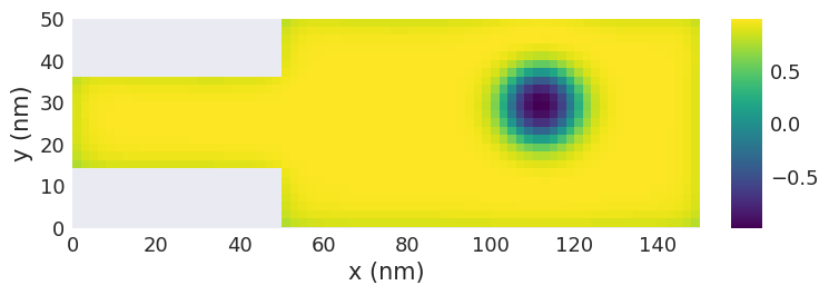
../../_images/getting-started_notebooks_dw-pair-conversion_26_0.png

We can create an interactive plot with a slider for the time to interactively investigate the conversion of the domain wall pair into a skyrmion.

[16]:

time_drive.hv(
    kdims=["x", "y"],
    scalar_kw={"clim": (-Ms, Ms), "cmap": "coolwarm"},
)

[16]:

`Table`#

We also get access to all tabular data recorded during the drive. The data is made available as pandas.Dataframe.

[17]:

time_drive.table.data

[17]:

	E	E_calc_count	max_dmdt	dE/dt	delta_E	average_u	E_exchange	max_spin_ang_exchange	stage_max_spin_ang_exchange	run_max_spin_ang_exchange	DMI_Cnv_z:dmi:Energy	E_uniaxialanisotropy	iteration	stage_iteration	stage	mx	my	mz	last_time_step	t
0	-3.138757e-19	61.0	5105.786662	1.131548e-09	1.234439e-22	400.0	7.819720e-19	24.981919	24.981919	24.981919	-1.791404e-18	6.955566e-19	8.0	8.0	0.0	-0.004356	0.001711	0.779309	1.146802e-13	1.000000e-12
1	-3.123365e-19	92.0	5393.820362	1.881778e-09	2.714936e-22	400.0	7.859070e-19	25.999114	25.999114	25.999114	-1.795166e-18	6.969222e-19	14.0	5.0	1.0	-0.007399	0.002527	0.779212	1.481817e-13	2.000000e-12
2	-3.101629e-19	129.0	5478.105937	2.410525e-09	1.525909e-22	400.0	7.908188e-19	26.839540	26.839540	26.839540	-1.800156e-18	6.991741e-19	21.0	6.0	2.0	-0.010058	0.002596	0.779103	6.371456e-14	3.000000e-12
3	-3.075651e-19	172.0	5775.596117	2.750961e-09	2.026333e-22	400.0	7.963184e-19	27.523018	27.523018	27.523018	-1.806035e-18	7.021517e-19	28.0	6.0	3.0	-0.012243	0.002078	0.779037	7.397143e-14	4.000000e-12
4	-3.046980e-19	209.0	6099.408455	2.938665e-09	1.417659e-22	400.0	8.020796e-19	27.968494	27.968494	27.968494	-1.812650e-18	7.058726e-19	35.0	6.0	4.0	-0.013915	0.001139	0.779058	4.838847e-14	5.000000e-12
...	...	...	...	...	...	...	...	...	...	...	...	...	...	...	...	...	...	...	...	...
195	-4.666219e-20	7786.0	6419.713717	2.798949e-10	1.373560e-23	400.0	1.222876e-18	29.279242	29.396487	33.740702	-1.937412e-18	6.678731e-19	1372.0	6.0	195.0	-0.007893	-0.008017	0.899229	5.094469e-14	1.960000e-10
196	-4.634379e-20	7829.0	6444.188876	2.763562e-10	1.564748e-23	400.0	1.222846e-18	29.358338	29.358338	33.740702	-1.936677e-18	6.674871e-19	1379.0	6.0	196.0	-0.007885	-0.008007	0.899298	6.044352e-14	1.970000e-10
197	-4.601751e-20	7866.0	6397.295744	2.905618e-10	1.926693e-23	400.0	1.222790e-18	29.418283	29.418283	33.740702	-1.935846e-18	6.670387e-19	1386.0	6.0	197.0	-0.007876	-0.007998	0.899383	7.101084e-14	1.980000e-10
198	-4.568193e-20	7909.0	6374.587943	3.124776e-10	1.795553e-23	400.0	1.222710e-18	29.397007	29.419861	33.740702	-1.934920e-18	6.665281e-19	1393.0	6.0	198.0	-0.007866	-0.007989	0.899482	5.961504e-14	1.990000e-10
199	-4.533615e-20	7946.0	6479.674566	3.377564e-10	2.490729e-23	400.0	1.222607e-18	29.301311	29.397007	33.740702	-1.933899e-18	6.659556e-19	1400.0	6.0	199.0	-0.007854	-0.007981	0.899595	7.547542e-14	2.000000e-10

200 rows × 20 columns

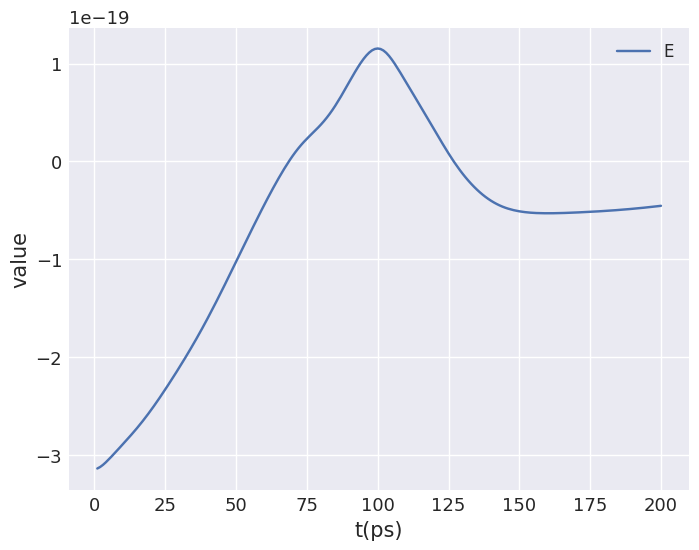
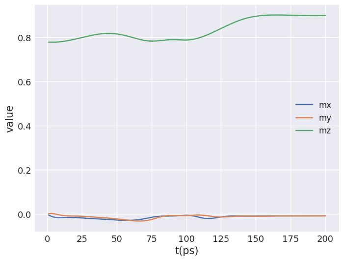
The table object provides a convenient plotting method. We can use it to visualise e.g. the total energy or the average magnetisation as a function of time. Ubermag, more precisely, ubermagtable automatically uses time for the x axis based on the metadata of the drive.

[18]:

time_drive.table.mpl(y=["E"])

../../_images/getting-started_notebooks_dw-pair-conversion_32_0.png

[19]:

time_drive.table.mpl(y=["mx", "my", "mz"])

../../_images/getting-started_notebooks_dw-pair-conversion_33_0.png

Derived quantities using callbacks#

We can also compute derived quantities for each time step and visualise them. As an example, we compute the topological charge density. Discretisedfield provides a function for this in discretisedfield.tools.

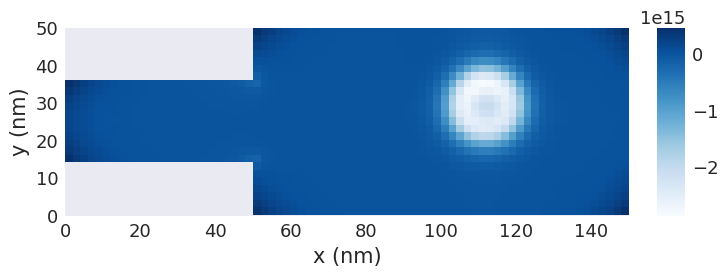
First, we compute the topolgical charge density for the final magnetisation state and plot it.

[20]:

final_magnetisation = time_drive[-1]
top_charge_last_step = df.tools.topological_charge_density(final_magnetisation.sel("z"))

top_charge_last_step.mpl.scalar(cmap="Blues")

../../_images/getting-started_notebooks_dw-pair-conversion_35_0.png

To compute a function for each time step, we use the register_callback method of Drive. We can pass in a function that will be called for each element of the drive. The function is only evaluated once we access an element of the drive. The register_callback method returns a new Drive object so that we still have access to the original data if required.

In this example we write a callback function that gets one magnetisation m and then selects a 2D slice normal to the z direction and computes the topological charge density.

[21]:

def top_charge_plane(m):
    return df.tools.topological_charge_density(m.sel("z"))


top_charge = time_drive.register_callback(top_charge_plane)

We can now plot the data of the new top_charge drive object. We manually compute suitable colour limits based on the topological charge in the final state to avoid changes of the colour range when moving the slider. (The plotting function always has only access to the current frame and would re-compute a suitable but changing colour range for each frame, which makes it difficult to judge the changes in topological charge.)

[22]:

c_min = top_charge_last_step.array.min()
c_max = top_charge_last_step.array.max()

top_charge.hv.scalar(kdims=["x", "y"], clim=(c_min, c_max))

[22]:

Analysing simulation results: Domain wall pair conversion#

Simulation#

Problem description#

References#

Solution#

Data analysis#

`Data`#

`Drive`#

`Table`#

Derived quantities using callbacks#

Conversion to `xarray.DataArray`#

Try online:

Try locally:

Analysing simulation results: Domain wall pair conversion#

Simulation#

Problem description#

References#

Solution#

Data analysis#

Data#

Drive#

Table#

Derived quantities using callbacks#

Conversion to xarray.DataArray#

Try online:

Try locally:

`Data`#

`Drive`#

`Table`#

Conversion to `xarray.DataArray`#