Hysteresis simulations

In this tutorial, we summarise some of the convenience methods offered by Ubermag that can be used for simulating hysteresis. Let us first define a simple system object. For details on how to define simulations, please refer to other tutorials.

import oommfc as mc
import discretisedfield as df
import micromagneticmodel as mm

region = df.Region(p1=(-50e-9, -50e-9, -50e-9), p2=(50e-9, 50e-9, 50e-9))
mesh = df.Mesh(region=region, cell=(5e-9, 5e-9, 5e-9))

system = mm.System(name="hysteresis")
system.energy = (
    mm.Exchange(A=1e-12)
    + mm.UniaxialAnisotropy(K=4e5, u=(0, 0, 1))
    + mm.DMI(D=1e-3, crystalclass="T")
)  # + mm.Demag()


def Ms_fun(point):
    x, y, z = point
    if x**2 + y**2 + z**2 <= 50e-9**2:
        return 1e6
    else:
        return 0


system.m = df.Field(mesh, nvdim=3, value=(0, 0, -1), norm=Ms_fun, valid="norm")

Now that we have system object we can simulate hysteresis using HysteresisDriver. Like all other drivers, HysteresisDriver has drive method. As input arguments it takes system object (as usual) and:

• Hmin - the starting value of magnetic field

• Hmin - the end value of magnetic field

• n - the number of points between Hmin and Hmax

For instance, let us say we want to simulate hysteresis between \(-1\,\text{T}\) and \(1\,\text{T}\) applied along the \(z\)-direction in steps of \(0.2\,\text{T}\). Accordingly, Hmin and Hmax are:

Hmin = (0, 0, -1 / mm.consts.mu0)
Hmax = (0, 0, 1 / mm.consts.mu0)

The number of steps n should be 21, so that the values of magnetic field are: \(-1\,\text{T}\), \(-0.9\,\text{T}\), \(-0.8\,\text{T}\), …, \(0.9\,\text{T}\), \(1\,\text{T}\), \(0.9\,\text{T}\), \(0.8\,\text{T}\), …, \(-0.9\,\text{T}\), \(-1\,\text{T}\).

n = 21

We can now create HysteresisDriver and drive the system.

hd = mc.HysteresisDriver()
hd.drive(system, Hmin=Hmin, Hmax=Hmax, n=n)

Running OOMMF (ExeOOMMFRunner)[2024/08/12 13:25]... (2.8 s)

After the simulation is complete, we can have a look at the last magnetisation step:

system.m.sel("y").mpl()

Similarly, table can be viewed:

system.table.data.head()

	max_mxHxm	E	delta_E	bracket_count	line_min_count	conjugate_cycle_count	cycle_count	cycle_sub_count	energy_calc_count	E_exchange	...	B_hysteresis	Bx_hysteresis	By_hysteresis	Bz_hysteresis	iteration	stage_iteration	stage	mx	my	mz
0	0.081239	-5.296243e-16	-2.958228e-31	9.0	9.0	1.0	8.0	7.0	19.0	1.178506e-19	...	1000.0	0.0	0.0	-1000.0	18.0	18.0	0.0	-7.579123e-20	-1.378022e-20	-0.998400
1	0.079335	-4.769135e-16	-8.874685e-31	16.0	15.0	2.0	15.0	6.0	33.0	1.301416e-19	...	900.0	0.0	0.0	-900.0	32.0	13.0	1.0	-5.512089e-20	-3.445056e-20	-0.998216
2	0.056329	-4.242133e-16	-9.860761e-32	23.0	22.0	3.0	22.0	6.0	48.0	1.445097e-19	...	800.0	0.0	0.0	-800.0	47.0	14.0	2.0	-4.065166e-19	2.067033e-20	-0.997999
3	0.086473	-3.715256e-16	-2.465190e-31	31.0	29.0	4.0	29.0	6.0	64.0	1.614662e-19	...	700.0	0.0	0.0	-700.0	62.0	14.0	3.0	-6.270001e-19	-8.612639e-20	-0.997739
4	0.053097	-3.188531e-16	-3.944305e-31	40.0	36.0	5.0	37.0	7.0	81.0	1.816966e-19	...	600.0	0.0	0.0	-600.0	78.0	15.0	4.0	1.067967e-19	2.756045e-20	-0.997422

5 rows × 26 columns

From the table, we can see at what external magnetic field the system was relaxed:

system.table.data["B_hysteresis"]

0     1000.0
1      900.0
2      800.0
3      700.0
4      600.0
5      500.0
6      400.0
7      300.0
8      200.0
9      100.0
10       0.0
11     100.0
12     200.0
13     300.0
14     400.0
15     500.0
16     600.0
17     700.0
18     800.0
19     900.0
20    1000.0
21     900.0
22     800.0
23     700.0
24     600.0
25     500.0
26     400.0
27     300.0
28     200.0
29     100.0
30       0.0
31     100.0
32     200.0
33     300.0
34     400.0
35     500.0
36     600.0
37     700.0
38     800.0
39     900.0
40    1000.0
Name: B_hysteresis, dtype: float64

The units of \(B\) are:

system.table.units["B_hysteresis"]

'mT'

Plotting hysteresis loop

Using Table object, we can plot different values as a function of external magnetic field. For that, as usual, we use mpl method. We have to specify to that method what do we want to have on the \(y\)-axis.

system.table.mpl(y=["mz"])

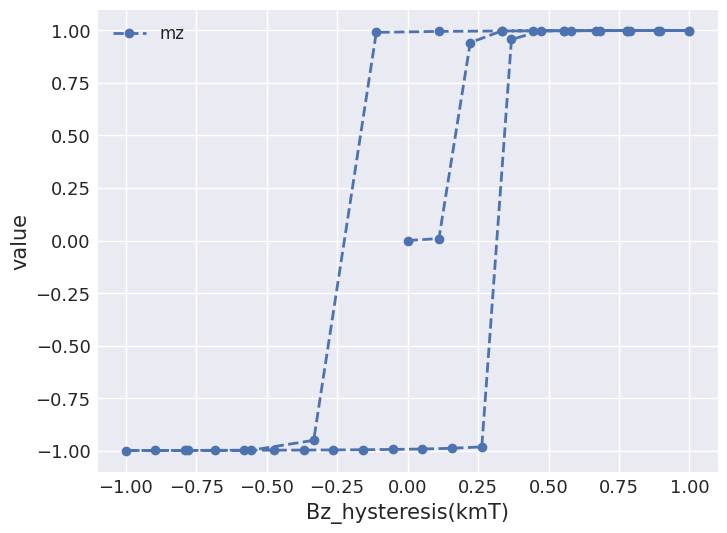
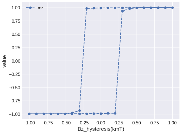
This does not look like a hysteresis loop as we expected. The reason is that on the horizontal axis we have the magnitude B by default, which is always positive. We can change that by passing Bz for x:

system.table.mpl(x="Bz_hysteresis", y=["mz"])

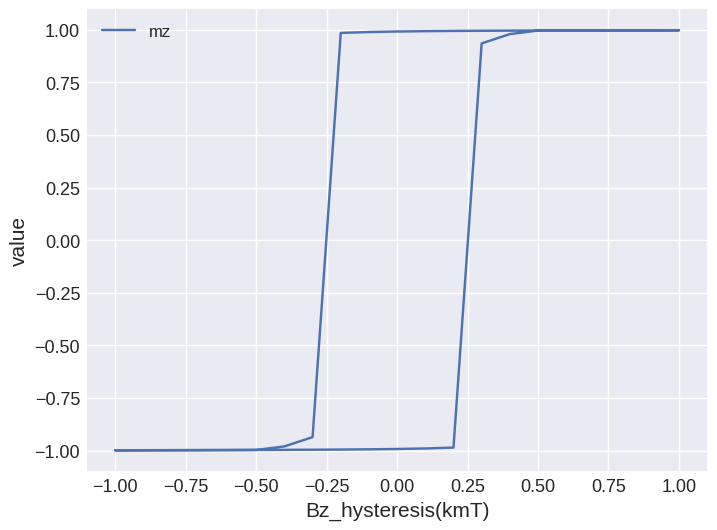
Table.mpl is based on matplotlib.pyplot.plot, so any keyword argument accepted by it can be passed:

system.table.mpl(
    x="Bz_hysteresis", y=["mz"], marker="o", linewidth=2, linestyle="dashed"
)

micromagneticdata analysis

We can also analyse magnetisation fields at different values of external magnetic field as well as building interactive plots using micromagneticdata package.

import micromagneticdata as md

We can create a data object by passing system’s name.

data = md.Data(name=system.name)

Now, we can have a look at all drives we did so far:

data.info

	drive_number	date	time	driver	adapter	Hsteps	n_threads
0	0	2024-08-12	13:25:57	HysteresisDriver	oommfc	[[[0, 0, -795774.7154594767], [0, 0, 795774.71...	None

There is only one drive with index 0. We can get if by indexing the data object:

drive = data[0]

The number of steps saved is:

drive.n

41

We can get an individual step by passing a value between 0 and 40 as an index:

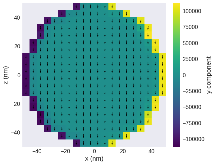
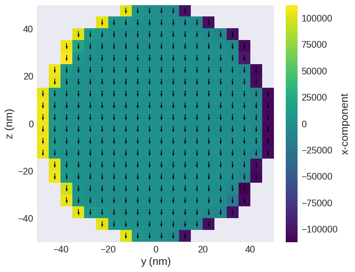
drive[0].sel("x").mpl()

We can also interactively plot all individual steps by using drive.hv. For more details on creating interactive plots, please refer to other tutorials.

drive.hv(kdims=["x", "y"])

Multi-step Hysteresis Drivers

Ubermag also provides a flexible version of a hysteresis driver which enables a hysteresis loop to be broken down into multiple curves. A list of hysteresis loop segments can be provided as an argument Hsteps. Each element of the list has the form (Hstart, Hend, n).

To see the power of this technique, we will first initialise the field and then perform a full hysteresis loop including the virgin curve.

system.m = df.Field(
    mesh,
    nvdim=3,
    value=lambda x: (0, 0, -1) if x[0] > 0 else (0, 0, 1),
    norm=Ms_fun,
    valid="norm",
)

hd = mc.HysteresisDriver()
hd.drive(system, Hsteps=[[(0, 0, 0), Hmax, 10], [Hmax, Hmin, 10], [Hmin, Hmax, 20]])

Running OOMMF (ExeOOMMFRunner)[2024/08/12 13:26]... (2.6 s)

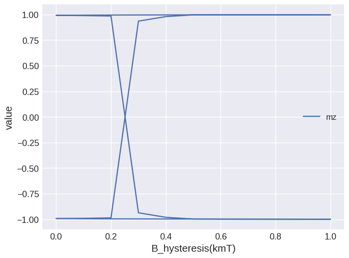
Finally we can plot the full curve.

system.table.mpl(
    x="Bz_hysteresis", y=["mz"], marker="o", linewidth=2, linestyle="dashed"
)