
Region basics#
An object on which finite difference mesh, and accordingly, finite difference field are based is Region. In this tutorial, we show how to define a region as well as some basic operations.
A region is can be defined in any number of spatial dimensions. It is always cuboidal and it can be defined by any two diagonally opposite corner points. For instance, let us assume we have a region in 3D Cartesian coordinates with edge lengths:
In order to define this region we need to choose two diagonally opposite corner points. There are many possibilities, but it is up to us which corner points we are going to choose as well as where we are going to position our region in Cartesian coordinate system. Most often, we choose either:
or
For simplicity, we are going to position \(p_{1}\) at the origin of the coordinate system.
For the three-dimensional Cartesian coordinates, we define points as length-3 tuples and pass them to Region object via p1 and p2 arguments.
[1]:
import discretisedfield as df  # df is here chosen to be an alias for discretisedfield

p1 = (0, 0, 0)
p2 = (100e-9, 50e-9, 20e-9)

region = df.Region(p1=p1, p2=p2)
(All units are SI and no prefixes are assumed. Therefore \(1 \,\text{nm}\) is 1e-9.)
The region is now defined. Now, we are going to have a look at some basic methods (functions) which are part of the Region object.
We can ask the region to give us the minimum and maximum points in the region.
[2]:
region.pmin
[2]:
array([0., 0., 0.])
[3]:
region.pmax
[3]:
array([1.e-07, 5.e-08, 2.e-08])
We can also ask the region for its dimensionality using attribute ndim.
[4]:
region.ndim
[4]:
3
In the above example \(p_\text{min} = p_{1}\) and \(p_\text{max} = p_{2}\), however, this is not the case every time. In general one could have chosen any two diagonally opposite points for \(p_{1}\) and \(p_{2}\) to define the region, for example, \({p}_{1} = (100\text{e}^{-9}, 0, 0)\) and \({p}_{1} = (0, 50\text{e}^{-9}, 20\text{e}^{-9})\) .
Now we can ask the region to give us the edge lengths of the region (based on \(p_{1}\) and \(p_{2}\) we used at the definition).
[5]:
region.edges
[5]:
array([1.e-07, 5.e-08, 2.e-08])
These lengths correspond to \(l_{x}\), \(l_{y}\), and \(l_{z}\) we discussed earlier.
Similarly, we can ask for a centre point in the region (cross section point of all diagonals).
[6]:
region.center
[6]:
array([5.0e-08, 2.5e-08, 1.0e-08])
Obviously, centre point we got is:
The volume of the region is:
[7]:
region.volume
[7]:
9.999999999999998e-23
This value is in \(\text{m}^{3}\) and it is calculated as
Now, let us say we have a point \(p\) and want to check if that point is in our region. We can do that using in. For instance, if our point is \(p = (2\,\text{nm}, 4\,\text{nm}, 1\,\text{nm})\), we can ask the region if point \(p\) is in it.
[8]:
p = (2e-9, 4e-9, 1e-9)

p in region
[8]:
True
As a result, we get bool (either True or False). This can be useful, when we want to use these expressions as conditions for some more complex functions. For example:
[9]:
if p in region:
    print("Point: I'm in! :)")
else:
    print("Point: I'm out! :(")
Point: I'm in! :)
On the other hand, we could have chosen a point which is outside of our region:
[10]:
(1e-9, 200e-9, 0) in region
[10]:
False
Sometimes we want to check if two regions are the same. We can do that using relational == operator. Let us define two regions: one which is the same to the one we have and one different:
[11]:
region_same = df.Region(p1=(0, 0, 0), p2=(100e-9, 50e-9, 20e-9))
region_different = df.Region(p1=(0, 0, 0), p2=(10e-9, 5e-9, 2e-9))
Now we can compare them:
[12]:
region == region_same
[12]:
True
[13]:
region == region_different
[13]:
False
Just like in operator, == returns bool. Similarly, we can ask if two regions are different:
[14]:
region != region_same
[14]:
False
[15]:
region != region_different
[15]:
True
Finally, we can ask the region object about its representation string:
[16]:
repr(region)
[16]:
"Region(pmin=[0.0, 0.0, 0.0], pmax=[1e-07, 5e-08, 2e-08], dims=['x', 'y', 'z'], units=['m', 'm', 'm'])"
In a Jupyter notebook we can also get an HTML representation.
[17]:
region
[17]:
- pmin = [0.0, 0.0, 0.0]
- pmax = [1e-07, 5e-08, 2e-08]
- dims = ['x', 'y', 'z']
- units = ['m', 'm', 'm']
From the representation we can see that a region has additional attributes dims and units. These have the default values shown above if we do not pass anything during initialisation.
[18]:
region.dims
[18]:
('x', 'y', 'z')
[19]:
region.units
[19]:
('m', 'm', 'm')
dims and units can be changed. This does not affect the actual data as units are only used as “labels”.
[20]:
region.units = ["nm", "nm", "nm"]
region.units
[20]:
('nm', 'nm', 'nm')
They can be reset to the default by passing None.
[21]:
region.units = None
region.units
[21]:
('m', 'm', 'm')
We can create a new region with custom dims and units.
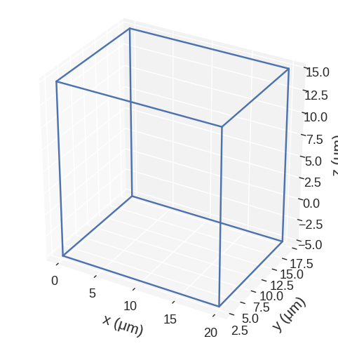
[22]:
region = df.Region(
    p1=(0, 0, 0), p2=(20, 20, 10), units=["μm", "μm", "μm"], dims=["x0", "x1", "x2"]
)
region
[22]:
- pmin = [0, 0, 0]
- pmax = [20, 20, 10]
- dims = ['x0', 'x1', 'x2']
- units = ['μm', 'μm', 'μm']
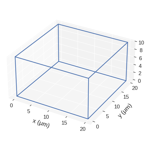
Regions can be plotted. There is a detailed notebook showing all the options. Here, we just use the defaults.
[23]:
region.mpl()
A regions has two methods scale and translate. Both optionally allow inplace operations.
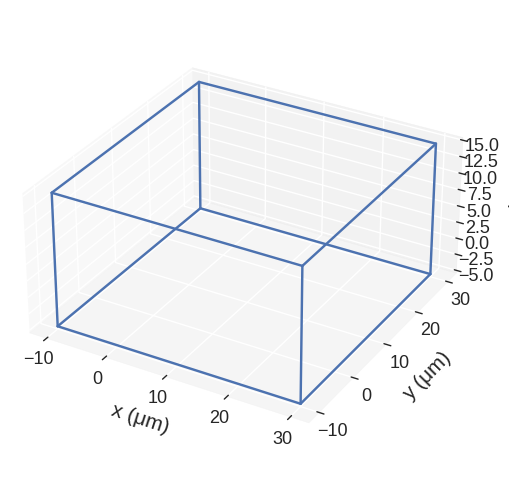
Scale#
[24]:
scaled = region.scale(2)
scaled
[24]:
- pmin = [-10.0, -10.0, -5.0]
- pmax = [30.0, 30.0, 15.0]
- dims = ['x0', 'x1', 'x2']
- units = ['μm', 'μm', 'μm']
[25]:
scaled.mpl()
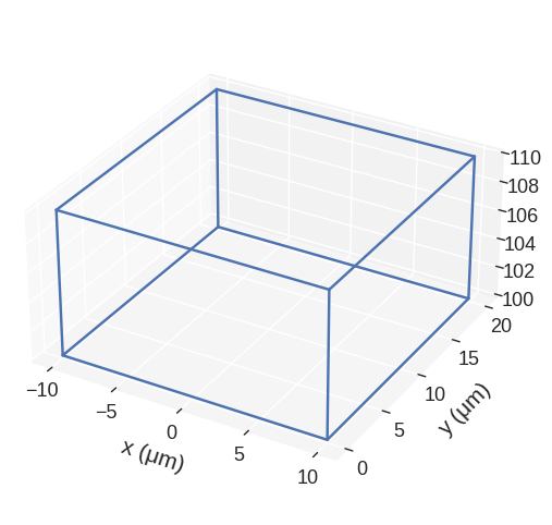
[26]:
region.translate((-10, 0, 100)).mpl()
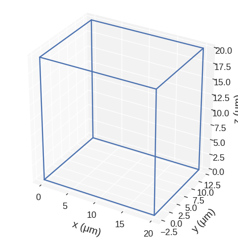
We can scale with different factors along different directions and pass in a reference_point that does not move when scaling. If not passed the center of the region is kept fixed.
[27]:
scaled = region.scale((1, 0.75, 2), reference_point=(-10, -10, 0))
scaled.mpl()
It is also possible to scale the region inplace.
[28]:
region.scale((1, 0.75, 2), inplace=True)
region.mpl()
Other dimensions#
Regions can have any dimension >= 1. Plotting is currently only supported for 3d regions.
A 1d region can be interpreted as a line.
[29]:
region_1d = df.Region(p1=0, p2=10)
region_1d
[29]:
- pmin = [0]
- pmax = [10]
- dims = ['x']
- units = ['m']
The dimensionality of a region can be obtained from the attribute ndim.
[30]:
region_1d.ndim
[30]:
1
A 2d region can be interpreted as a plane.
[31]:
df.Region(p1=(0, 0), p2=(10, 20))
[31]:
- pmin = [0, 0]
- pmax = [10, 20]
- dims = ['x', 'y']
- units = ['m', 'm']
For dimension larger than three the default for dims changes from [x, y, z] to x0 to xn-1.
[32]:
df.Region(p1=(1, 2, 3, 4), p2=(10, 20, 30, 40))
[32]:
- pmin = [1, 2, 3, 4]
- pmax = [10, 20, 30, 40]
- dims = ['x0', 'x1', 'x2', 'x3']
- units = ['m', 'm', 'm', 'm']