Magnetisation field

One of the main objects, which we have to be specify as a part of the micromagnetic system is the magnetisation field \(\mathbf{M}\). In Ubermag, by defining the magnetisation field, the mesh, the geometry of the sample, as well as the magnetisation saturation \(M_\text{s}\) are defined.

The Ubermag package we use to define finite difference regions, meshes, and fields is discretisedfield and we have to import it before we use it.

import discretisedfield as df  # df is just a shorter name

Region

In finite differences, the region on which the mesh and the field are specified is always cuboidal. In order to define a mesh, two points \(p_{1}\) and \(p_{2}\) must be passed to discretisedfield.Region. Those points correspond to two points between which the region spans.

For instance, if we want to define the following region:

\[x \in [0, 100]\,\text{nm}\]

\[y \in [-20, 20]\,\text{nm}\]

\[z \in [0, 10]\,\text{nm}\]

two points we need to pass are:

\[p_\text{1} = (0 \,\text{nm}, -20 \,\text{nm}, 0 \,\text{nm})\]

\[p_\text{2} = (100 \,\text{nm}, 20 \,\text{nm}, 10 \,\text{nm})\]

In Ubermag, points are defined as sequences, for instance, tuples. The length of these sequences gives the number of spatial dimensions that are defined in the region. Accordingly, the region we want is:

p1 = (0, -20e-9, 0)  # point 1
p2 = (100e-9, 20e-9, 10e-9)  # point 2

region = df.Region(p1=p1, p2=p2)

There are several quantitites we can ask the region object for.

region.pmin  # minimum coordinate in the region

array([ 0.e+00, -2.e-08,  0.e+00])

region.pmax  # maximum coordinate in the region

array([1.e-07, 2.e-08, 1.e-08])

region.centre  # the region centre

array([5.e-08, 0.e+00, 5.e-09])

region.edges  # edge lengths of the region

array([1.e-07, 4.e-08, 1.e-08])

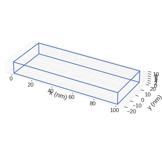
We can visualise the region e.g. using matplotlib mpl().

region.mpl()

Mesh

After the region is defined, we need to discretise it in order to define a mesh. There are two ways how a region can be discretised - by passing:

1. Discretisation cell size (cell), or

2. Number of discretisation cells in all three directions (n).

Let us say we want to discretise our region in cells of size \((10\,\text{nm}, 10\,\text{nm}, 10\,\text{nm})\). Then, we pass the region and the cell size to Mesh class.

cell = (10e-9, 10e-9, 10e-9)  # discretisation cell
mesh = df.Mesh(region=region, cell=cell)  # mesh definition

We can then inspect some basic parameters of the mesh.

mesh.n  # number of discretisation cells

array([10,  4,  1])

len(mesh)  # total number of discretisation cells

40

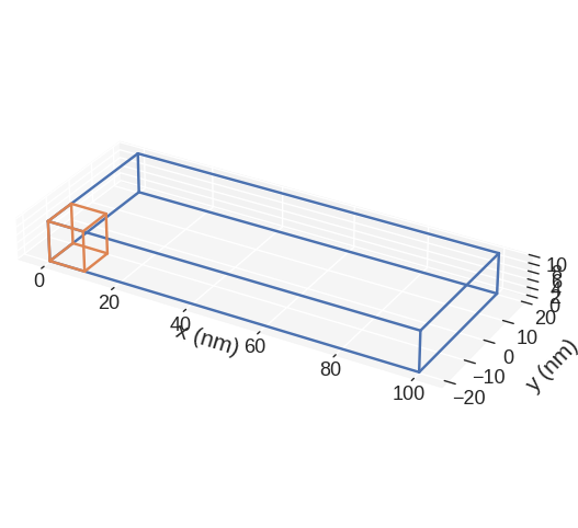
We can visualise the mesh e.g. using matplotlib mpl().

mesh.mpl()

When we have the mesh object created, we can access the region using . operator. For instance:

mesh.region.centre

array([5.e-08, 0.e+00, 5.e-09])

Field

After we defined the mesh, we can define a finite difference field. For that, we use Field class. We must provide the following 3 mandatory parameters:

1. mesh (discretisedfield.Mesh),

2. dimension of the value/vector (e.g. nvdim=1 for scalar, nvdim=3 for three dimensional vector),

3. value of the field (value).

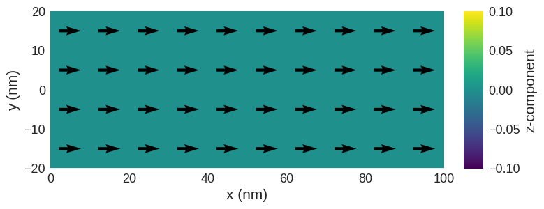
For instance, let us define a 3D-vector field (nvdim=3) that is uniform in the \(x\)-direction value=(1, 0, 0) direction.

m = df.Field(mesh, nvdim=3, value=(1, 0, 0))

A simple visualisation of the field in \(z\)-slice through the middle is:

m.sel('z').mpl()

The average value of the field is:

m.mean()

array([1., 0., 0.])

We can specify the norm of the field, by passing norm parameter. In the case of magnetisation, norm corresponds to magnetisation saturation \(M_\text{s}\).

Ms = 8e6  # A/m
m = df.Field(mesh, nvdim=3, value=(0, 0, 1), norm=Ms)

Now, if we have a look at the average:

m.mean()

array([      0.,       0., 8000000.])

Spatially varying field value

When we defined a uniform vector field, we used a tuple value=(1, 0, 0) to define its value. However, we can also pass a callable (e.g. Python function) if we want to define a non-uniform field. This function takes the coordinate of the mesh cell as an input, and returns a value that the field should have at that point. The function must be defined at all points in the mesh.

def m_value(point):
    x, y, z = point  # unpack position into individual components
    if y > 0:
        return (1, 0, 0)
    else:
        return (-1, 1, 0)

m = df.Field(mesh, nvdim=3, value=m_value)

Now, we can plot it using mpl.

m.sel('z').mpl()

The field object can be treated as a callable - if we pass a point to the function, it will return the vector value of the field at that location:

point = (0, -10e-9, 0)
m(point)

array([-1.,  1.,  0.])

point = (0, 10e-9, 0)
m(point)

array([1., 0., 0.])

m(m.mesh.region.centre)

array([1., 0., 0.])

Spatially varying \(M_\mathrm{s}\)

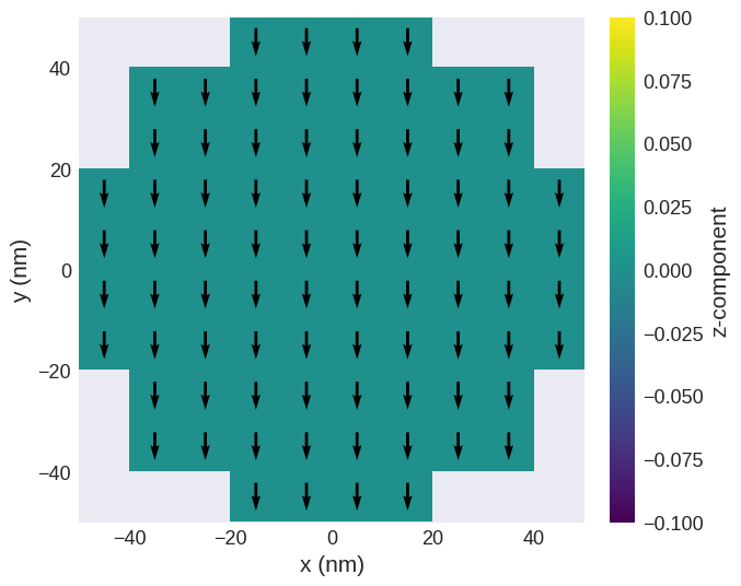
By defining a norm of a field, we can specify different geometries. More precisely, we can set \(M_\text{s}=0\) where no magnetic material is present. For instance, let us assume we want to define a sphere of radius \(r=50\,\text{nm}\), discrectised by 10 cells in each direction, and magnetise it in the negative \(y\) direction. We can also set where we want the field to be valid, for example where the norm is not zero.

r = 50e-9
n = (10, 10, 10)
region = df.Region(p1=(-r, -r, -r), p2=(r, r, r))
mesh = df.Mesh(region=region, n=n)

def Ms_value(point):
    x, y, z = point
    if x**2 + y**2 + z**2 < r**2:
        return Ms
    else:
        return 0

m = df.Field(mesh, nvdim=3, value=(0, -1, 0), norm=Ms_value, valid="norm")

m.sel('z').mpl()

Example

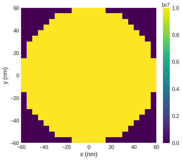
Let us define a thin-film disk sample of thickness \(t = 10 \,\text{nm}\) and diameter \(d = 120 \,\text{nm}\). The saturation magnetisation \(M_\mathrm{s} = 10^{7}\mathrm{A/m}\). The disk is centred at the origin (0, 0, 0) and the magnetisation is \(\mathbf{m} = (1, 0, 0)\) at all mesh points.

t = 10e-9  # thickness (m)
d = 120e-9  # diameter (m)
cell = (5e-9, 5e-9, 5e-9)  # discretisation cell size (m)
Ms = 1e7  # saturation magnetisation (A/m)

region = df.Region(p1=(-d/2, -d/2, -t/2), p2=(d/2, d/2, t/2))
mesh = df.Mesh(region=region, cell=cell)

def Ms_value(point):
    x, y, z = point
    if (x**2 + y**2)**0.5 < d/2:
        return Ms
    else:
        return 0

m = df.Field(mesh, nvdim=3, value=(1, 0, 0), norm=Ms_value)

m.norm.sel('z').mpl()

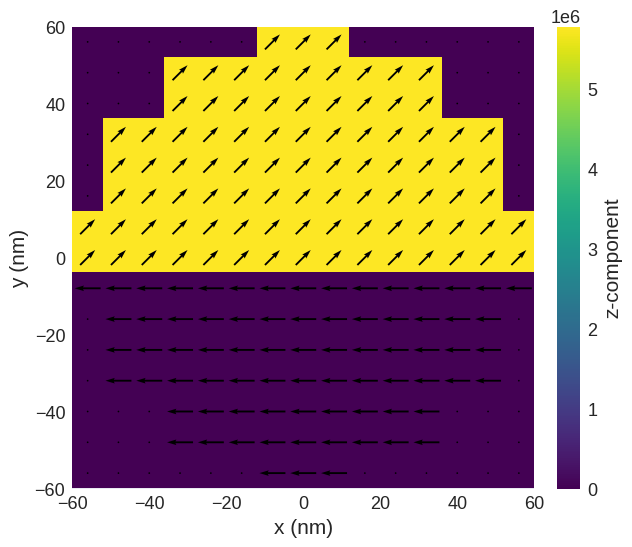
Now, let us say we want to extend the solution from the previous example so that the magnetisation is:

\[\begin{split}\mathbf{m} = \begin{cases} (-1, 0, 0) & \text{for } y \le 0 \\ (1, 1, 1) & \text{for } y > 0 \end{cases}\end{split}\]

with saturation magnetisation \(M_\text{s} = 10^{7} \,\text{A}\,\text{m}^{-1}\).

def m_value(pos):
    x, y, z = pos
    if y <= 0:
        return (-1, 0, 0)
    else:
        return (1, 1, 1)

m = df.Field(mesh, nvdim=3, value=m_value, norm=Ms_value)

m.sel('z').resample((15, 15)).mpl()

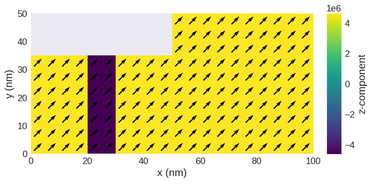
Exercise

Define the following sample with \(10\,\text{nm}\) thickness:

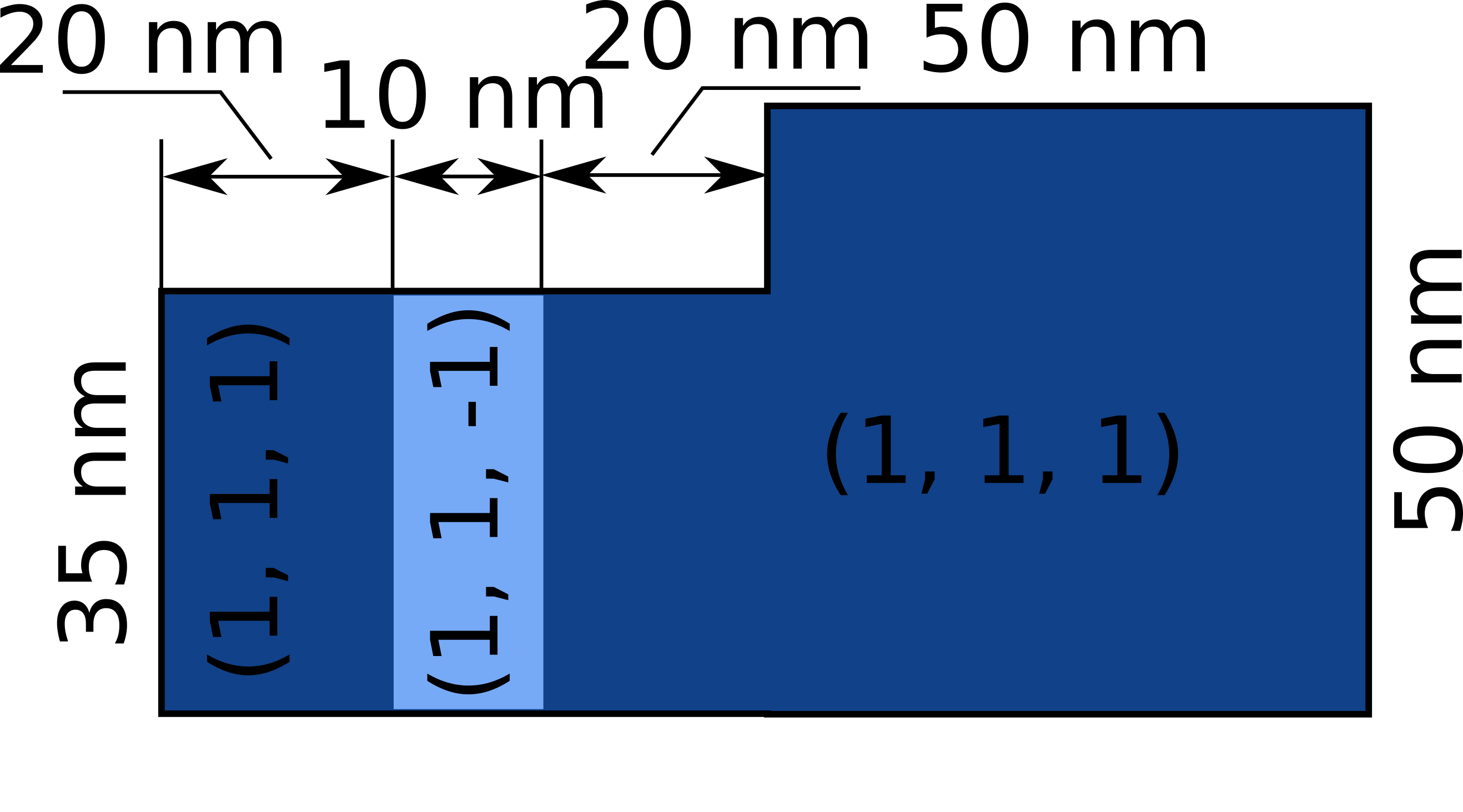
The magnetisation saturation is \(M_\mathrm{s} = 8 \times 10^{6} \,\mathrm{A}\,\mathrm{m}^{-1}\) and the magnetisation direction is as shown in the figure.

Solution

cell = (5e-9, 5e-9, 5e-9)  # discretisation cell size (m)
Ms = 8e6  # saturation magnetisation (A/m)

region = df.Region(p1=(0, 0, 0), p2=(100e-9, 50e-9, 10e-9))
mesh = df.Mesh(region=region, cell=cell)

def Ms_value(pos):
    x, y, z = pos
    if x < 50e-9 and y > 35e-9:
        return 0
    else:
        return Ms

def m_value(pos):
    x, y, z = pos
    if 20e-9 < x <= 30e-9:
        return (1, 1, -1)
    else:
        return (1, 1, 1)

m = df.Field(mesh, nvdim=3, value=m_value, norm=Ms_value, valid="norm")

m.sel('z').mpl()