Dynamics equation#

The dynamics of magnetisation field $\mathbf{m}$, without external excitations (e.g. spin-polarised current) is governed by the Landau-Lifshitz-Gilbert (LLG) equation

\[\frac{d\mathbf{m}}{dt} = \underbrace{-\gamma_{0}(\mathbf{m} \times \mathbf{H}_\text{eff})}_\text{precession} + \underbrace{\alpha\left(\mathbf{m} \times \frac{d\mathbf{m}}{dt}\right)}_\text{damping},\]

where $\gamma_{0} = \mu_{0}\gamma$ is the gyromagnetic ratio, $\alpha$ is the Gilbert damping, and $\mathbf{H}_\text{eff} = -\frac{1}{\mu_{0}M_\text{s}}\frac{\delta w(\mathbf{m})}{\delta \mathbf{m}}$ is the effective field. It consists of two terms: precession and damping. In this tutorial, we will explore some basic properties of this equation to understand how to define it in simulations.

Macrospin#

We will study the simplest “zero-dimensional” case - macrospin. In the first step, after we import necessary modules and create the mesh which consists of a single discretisation cell.

[1]:

import oommfc as mc
import discretisedfield as df
import micromagneticmodel as mm

# Define a macrospin mesh (i.e. one discretisation cell).
p1 = (0, 0, 0)  # first point of the mesh domain (m)
p2 = (1e-9, 1e-9, 1e-9)  # second point of the mesh domain (m)
n = (1, 1, 1)  # discretisation cell size (m)

region = df.Region(p1=p1, p2=p2)
mesh = df.Mesh(region=region, n=n)

Now, we can create a micromagnetic system object.

[2]:

system = mm.System(name='macrospin')

Let us assume we have a simple Hamiltonian which consists of only Zeeman energy term

\[w = -\mu_{0}M_\text{s}\mathbf{m}\cdot\mathbf{H},\]

where $M_\text{s}$ is the saturation magnetisation, $\mu_{0}$ is the magnetic constant, and $\mathbf{H}$ is the external magnetic field. We apply the external magnetic field with magnitude $H = 2 \times 10^{6} \,\text{A}\,\text{m}^{-1}$ in the positive $z$ direction.

[3]:

H = (0, 0, 2e6)  # external magnetic field (A/m)
system.energy = mm.Zeeman(H=H)

Dynamics simulation#

In the next step we can define the system’s dynamics. Let us assume we have $\gamma_{0} = 2.211 \times 10^{5} \,\text{m}\,\text{A}^{-1}\,\text{s}^{-1}$ and $\alpha=0.1$.

[4]:

gamma0 = 2.211e5  # gyromagnetic ratio (m/As)
alpha = 0.1  # Gilbert damping

system.dynamics = mm.Precession(gamma0=gamma0) + mm.Damping(alpha=alpha)

To check what is our dynamics equation:

[5]:

system.dynamics

[5]:

$-\frac{\gamma_{0}}{1 + \alpha^{2}} \mathbf{m} \times \mathbf{H}_\text{eff}-\frac{\gamma_{0} \alpha}{1 + \alpha^{2}} \mathbf{m} \times (\mathbf{m} \times \mathbf{H}_\text{eff})$

Before we start running time evolution simulations, we need to initialise the magnetisation. In this case, our magnetisation is pointing in the positive $x$ direction with $M_\text{s} = 8 \times 10^{6} \,\text{A}\,\text{m}^{-1}$. The magnetisation is defined using Field class from the discretisedfield package we imported earlier.

[6]:

initial_m = (1, 0, 0)  # vector in x direction
Ms = 8e6  # magnetisation saturation (A/m)

system.m = df.Field(mesh, nvdim=3, value=initial_m, norm=Ms)

Now, we can run the time evolution using TimeDriver for $t=0.1 \,\text{ns}$ and save the magnetisation configuration in $n=200$ steps.

[7]:

td = mc.TimeDriver()
td.drive(system, t=0.1e-9, n=200)

Running OOMMF (ExeOOMMFRunner)[2023/10/23 15:56]... (0.8 s)

Simulation results#

How different system parameters vary with time, we can inspect by showing the system’s datatable.

[8]:

system.table.data

[8]:

	E	E_calc_count	max_dm/dt	dE/dt	delta_E	E_zeeman	iteration	stage_iteration	stage	mx	my	mz	last_time_step	t
0	-4.400762e-22	37.0	25204.415522	-8.798712e-10	-3.269612e-22	-4.400762e-22	6.0	6.0	0.0	0.975901	0.217115	0.021888	3.715017e-13	5.000000e-13
1	-8.797309e-22	44.0	25186.311578	-8.786077e-10	-4.396547e-22	-8.797309e-22	8.0	1.0	1.0	0.904810	0.423562	0.043754	5.000000e-13	1.000000e-12
2	-1.318544e-21	51.0	25156.186455	-8.765071e-10	-4.388134e-22	-1.318544e-21	10.0	1.0	2.0	0.790286	0.609218	0.065579	5.000000e-13	1.500000e-12
3	-1.756100e-21	58.0	25114.112032	-8.735776e-10	-4.375555e-22	-1.756100e-21	12.0	1.0	3.0	0.638055	0.765021	0.087341	5.000000e-13	2.000000e-12
4	-2.191985e-21	65.0	25060.188355	-8.698302e-10	-4.358857e-22	-2.191985e-21	14.0	1.0	4.0	0.455710	0.883427	0.109020	5.000000e-13	2.500000e-12
...	...	...	...	...	...	...	...	...	...	...	...	...	...	...
195	-2.009865e-20	1402.0	690.438568	-6.602614e-13	-3.374608e-25	-2.009865e-20	396.0	1.0	195.0	0.013011	-0.024099	0.999625	5.000000e-13	9.800000e-11
196	-2.009897e-20	1409.0	675.493807	-6.319876e-13	-3.230101e-25	-2.009897e-20	398.0	1.0	196.0	0.017545	-0.020251	0.999641	5.000000e-13	9.850000e-11
197	-2.009928e-20	1416.0	660.872303	-6.049242e-13	-3.091780e-25	-2.009928e-20	400.0	1.0	197.0	0.021059	-0.015612	0.999656	5.000000e-13	9.900000e-11
198	-2.009958e-20	1423.0	646.567078	-5.790193e-13	-2.959381e-25	-2.009958e-20	402.0	1.0	198.0	0.023428	-0.010435	0.999671	5.000000e-13	9.950000e-11
199	-2.009986e-20	1430.0	632.571305	-5.542233e-13	-2.832649e-25	-2.009986e-20	404.0	1.0	199.0	0.024591	-0.004988	0.999685	5.000000e-13	1.000000e-10

200 rows × 14 columns

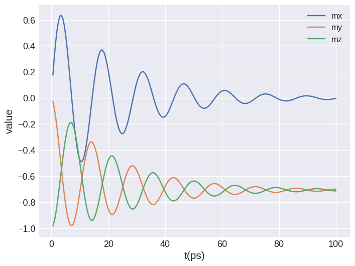
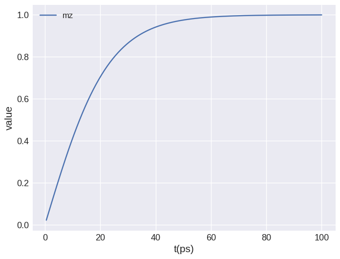
However, in our case it is much more informative if we plot the time evolution of magnetisation $z$ component $m_{z}(t)$.

[9]:

system.table.mpl(y=['mz'])

../../_images/getting-started_notebooks_dynamics-equation_17_0.png

Similarly, we can plot all three magnetisation components

[10]:

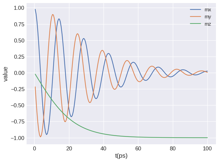
system.table.mpl(y=['mx', 'my', 'mz'])

../../_images/getting-started_notebooks_dynamics-equation_19_0.png

We can see that after some time the macrospin aligns parallel to the external magnetic field in the $z$ direction. We can also have a look at the dynamics using an interactive plot.

Exercise 1#

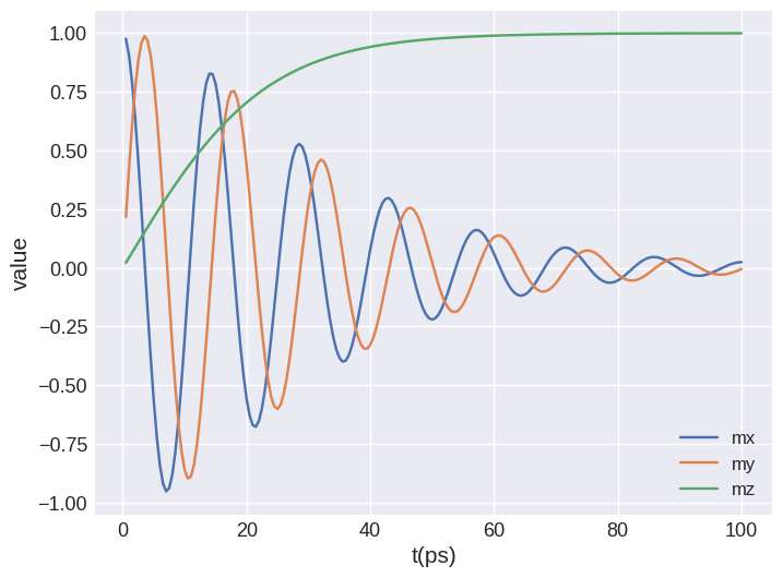
Modify Gilbert damping and set it to $\alpha=0.005$ and see what happens with the dynamics.

Solution

[11]:

system.dynamics.damping.alpha = 0.005
system.m = df.Field(mesh, nvdim=3, value=initial_m, norm=Ms)

td.drive(system, t=0.1e-9, n=200)

system.table.mpl(y=['mx', 'my', 'mz'])

Running OOMMF (ExeOOMMFRunner)[2023/10/23 15:56]... (0.6 s)

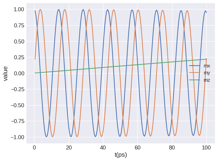
../../_images/getting-started_notebooks_dynamics-equation_22_1.png

Exercise 2#

Repeat the simulation with $\alpha=0.1$ and $\mathbf{H} = (0, 0, -2\times 10^{6})\,\text{A}\,\text{m}^{-1}$.

Solution

[12]:

system.energy.zeeman.H = (0, 0, -2e6)
system.dynamics.damping.alpha = 0.1
system.m = df.Field(mesh, nvdim=3, value=initial_m, norm=Ms)

td.drive(system, t=0.1e-9, n=200)

system.table.mpl(y=['mx', 'my', 'mz'])

Running OOMMF (ExeOOMMFRunner)[2023/10/23 15:56]... (0.6 s)

../../_images/getting-started_notebooks_dynamics-equation_24_1.png

Exercise 3#

Keep using $\alpha=0.1$. Change the field from H = (0, 0, -2e6) to H = (0, -1.41e6, -1.41e6), and plot $m_x(t)$, $m_y(t)$ and $m_z(t)$ as above. Can you explain the (initially non-intuitive) output?

[13]:

system.energy.zeeman.H = (0, -1.41e6, -1.41e6)

td.drive(system, t=0.1e-9, n=200)

system.table.mpl(y=['mx', 'my', 'mz'])

Running OOMMF (ExeOOMMFRunner)[2023/10/23 15:56]... (0.7 s)

../../_images/getting-started_notebooks_dynamics-equation_26_1.png