Deriving energy values

In this tutorial, we show how derived fields and values can be computed after the micromagnetic system is defined.

Simulation

First of all, as usual, we import oommfc and discretisedfield.

import oommfc as oc
import discretisedfield as df
import micromagneticmodel as mm

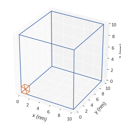
We define the cube mesh with edge length \(10 \,\text{nm}\) and cell discretisation edge \(1 \,\text{nm}\).

mesh = df.Mesh(p1=(0, 0, 0), p2=(10e-9, 10e-9, 10e-9), cell=(1e-9, 1e-9, 1e-9))
mesh.mpl()

Now we define the system object and its Hamiltonian.

system = mm.System(name='system')

A = 1e-11
H = (0.1/mm.consts.mu0, 0, 0)
K = 1e3
u = (1, 1, 1)
system.energy = (mm.Exchange(A=A)
                 + mm.Demag()
                 + mm.Zeeman(H=H)
                 + mm.UniaxialAnisotropy(K=K, u=u))

system.energy

$- A \mathbf{m} \cdot \nabla^{2} \mathbf{m}-\frac{1}{2}\mu_{0}M_\text{s}\mathbf{m} \cdot \mathbf{H}_\text{d}-\mu_{0}M_\text{s} \mathbf{m} \cdot \mathbf{H}-K (\mathbf{m} \cdot \mathbf{u})^{2}$

We will now intialise the system in \((0, 0, 1)\) direction with \(M_\text{s} = 8\times 10^{5} \,\text{A/m}\) and relax the magnetisation.

Ms = 8e5
system.m = df.Field(mesh, nvdim=3, value=(0, 0, 1), norm=Ms)

Effective field

All computations are performed using oc.compute, where oc is the micromagnetic calculator we choose at import. compute function takes two arguments:

1. Property we want to compute

2. System object

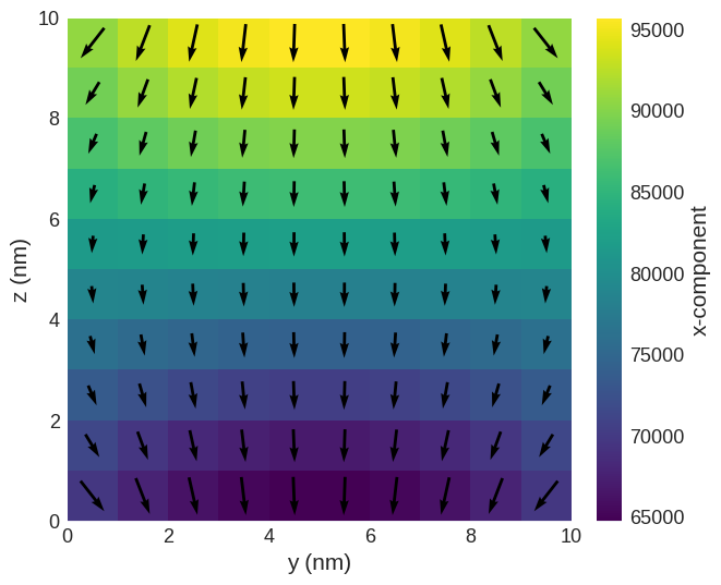
Total effective field is:

oc.compute(system.energy.effective_field, system).sel('x').mpl()

Running OOMMF (ExeOOMMFRunner)[2023/10/23 16:06]... (0.4 s)

Similarly, the individual exchange effective field is:

Hex_eff = oc.compute(system.energy.exchange.effective_field, system)

Running OOMMF (ExeOOMMFRunner)[2023/10/23 16:06]... (0.2 s)

Because we initialised the system with the uniform state, we expect this effective field to be zero.

Hex_eff.mean()

array([0., 0., 0.])

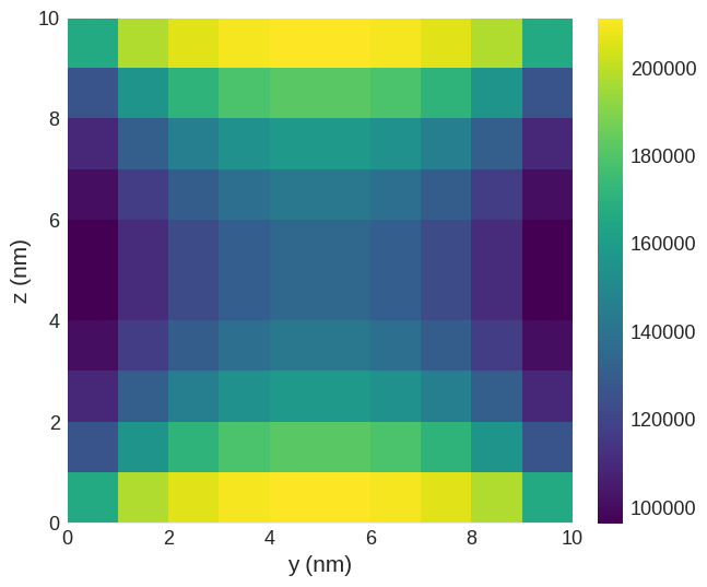
The energy density is:

w = oc.compute(system.energy.density, system)
w.sel('x').mpl()

Running OOMMF (ExeOOMMFRunner)[2023/10/23 16:06]... (0.2 s)

Similarly, the energy (volume integral of energy density) is:

E = oc.compute(system.energy.energy, system)
print(f'The energy of the system is {E} J.')

Running OOMMF (ExeOOMMFRunner)[2023/10/23 16:06]... (0.2 s)
The energy of the system is 1.3470795322e-19 J.

Relax the system

md = oc.MinDriver()
md.drive(system)

Running OOMMF (ExeOOMMFRunner)[2023/10/23 16:06]... (0.4 s)

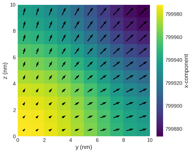
Compute the energy (and demonstrate that the energy decreased) and plot its magnetisation:

E = oc.compute(system.energy.energy, system)
print("The system's energy is {} J.".format(E))

system.m.sel('x').mpl()

Running OOMMF (ExeOOMMFRunner)[2023/10/23 16:06]... (0.2 s)
The system's energy is 5.35285533145e-20 J.

Computing energies of individual term

For instance, the exchange energy is:

oc.compute(system.energy.exchange.energy, system)

Running OOMMF (ExeOOMMFRunner)[2023/10/23 16:06]... (0.4 s)

1.12170191751e-21

We can also check the sum of all individual energy terms and check if it the same as the total energy.

total_energy = 0
for term in system.energy:
    total_energy += oc.compute(term.energy, system)

print("The sum of energy terms is {} J.".format(total_energy))
print("The system's energy is {} J.".format(oc.compute(system.energy.energy, system)))

Running OOMMF (ExeOOMMFRunner)[2023/10/23 16:06]... (0.3 s)
Running OOMMF (ExeOOMMFRunner)[2023/10/23 16:06]... (0.3 s)
Running OOMMF (ExeOOMMFRunner)[2023/10/23 16:06]... (0.2 s)
Running OOMMF (ExeOOMMFRunner)[2023/10/23 16:06]... (0.2 s)
The sum of energy terms is 5.352855331462e-20 J.
Running OOMMF (ExeOOMMFRunner)[2023/10/23 16:06]... (0.3 s)
The system's energy is 5.35285533145e-20 J.