
Periodic boundary conditions#
In this tutorial, we compute and relax a skyrmion in an interfacial-DMI (Cnv) material in a part of an infinitely large thin film.
[1]:
import oommfc as mc
import discretisedfield as df
import micromagneticmodel as mm
We define mesh in cuboid through corner points p1 and p2, and discretisation cell size cell.
[2]:
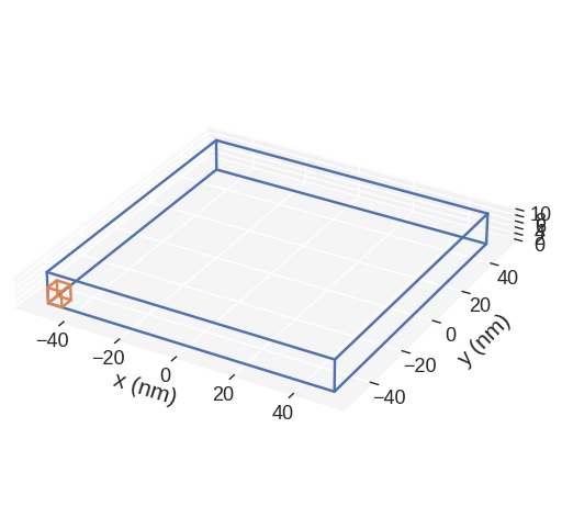
region = df.Region(p1=(-50e-9, -50e-9, 0), p2=(50e-9, 50e-9, 10e-9))
mesh = df.Mesh(region=region, cell=(5e-9, 5e-9, 5e-9), bc="xy")
Here bc="xy" means that we have periodic boundary conditions along the x and y directions. The mesh we defined is:
[3]:
mesh.mpl()
Now, we can define the system object by first setting up the Hamiltonian:
[4]:
system = mm.System(name="skyrmion")

system.energy = (
    mm.Exchange(A=1.6e-11)
    + mm.DMI(D=4e-3, crystalclass="Cnv_z")
    + mm.UniaxialAnisotropy(K=0.2e6, u=(0, 0, 1))
    + mm.Zeeman(H=(0, 0, 1e5))
)

system.energy
[4]:
$- A \mathbf{m} \cdot \nabla^{2} \mathbf{m}+ D ( \mathbf{m} \cdot \nabla m_{z} - m_{z} \nabla \cdot \mathbf{m} )-K (\mathbf{m} \cdot \mathbf{u})^{2}-\mu_{0}M_\text{s} \mathbf{m} \cdot \mathbf{H}$
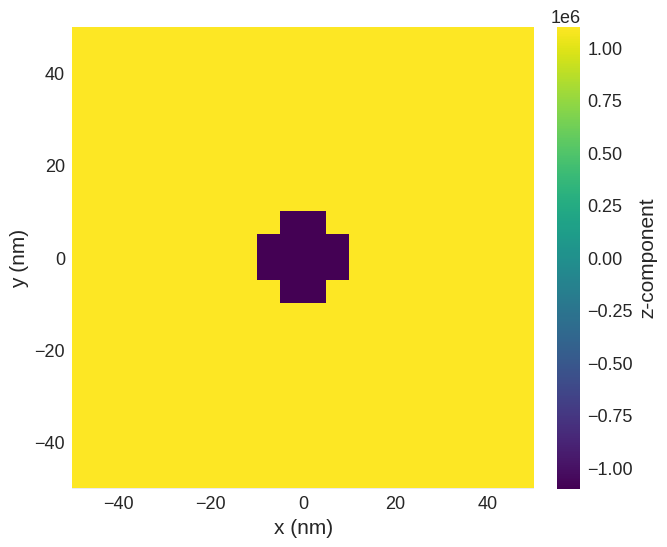
Now, we need to define a function to define the initial magnetisation which is going to relax to skyrmion.
[5]:
def m_init(pos):
    """Function to set initial magnetisation direction:
    -z inside cylinder (r=10nm),
    +z outside cylinder.
    y-component to break symmetry.

    """
    x, y, z = pos
    if (x**2 + y**2) ** 0.5 < 10e-9:
        return (0, 0, -1)
    else:
        return (0, 0, 1)


system.m = df.Field(mesh, nvdim=3, value=m_init, norm=1.1e6)
The initial magnetsation is:
[6]:
system.m.sel("z").mpl()
/home/mlang/miniconda3/envs/ubermagdev310/lib/python3.10/site-packages/matplotlib/quiver.py:645: RuntimeWarning: divide by zero encountered in scalar divide
  length = a * (widthu_per_lenu / (self.scale * self.width))
/home/mlang/miniconda3/envs/ubermagdev310/lib/python3.10/site-packages/matplotlib/quiver.py:645: RuntimeWarning: invalid value encountered in multiply
  length = a * (widthu_per_lenu / (self.scale * self.width))
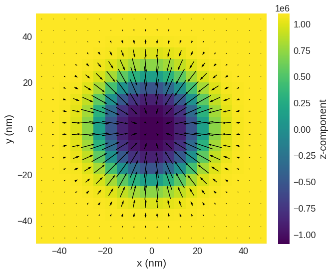
Finally we can minimise the energy and plot the magnetisation.
[7]:
# minimize the energy
md = mc.MinDriver()
md.drive(system)

# Plot relaxed configuration: vectors in z-plane
system.m.sel("z").mpl()
Running OOMMF (ExeOOMMFRunner)[2023/10/23 16:08]... (0.4 s)
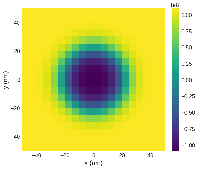
[8]:
# Plot z-component only:
system.m.z.sel("z").mpl()
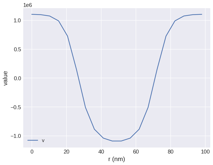
Finally we can sample and plot the magnetisation along the line:
[9]:
system.m.z.line(p1=(-49e-9, 0, 0), p2=(49e-9, 0, 0), n=20).mpl()
Finally let us compute the skyrmion number
\[S = \frac{1}{4\pi}\int\mathbf{m}\cdot\left(\frac{\partial \mathbf{m}}{\partial x} \times \frac{\partial \mathbf{m}}{\partial y}\right)dxdy\]
[10]:
import math

m = system.m.orientation.sel("z")

1 / (4 * math.pi) * (m.dot(m.diff("x").cross(m.diff("y")))).integrate()
[10]:
array([-0.92414447])
[11]:
import discretisedfield.tools as dft

dft.topological_charge(system.m.sel("z"))
[11]:
-0.9241444720743723
[12]:
dft.topological_charge(system.m.sel("z"), method="berg-luescher")
[12]:
-1.0001397845194369