MplField

class discretisedfield.plotting.MplField(field)

Matplotlib-based plotting methods.

Before the field can be plotted, it must be ensured that it is defined on two dimensional geometry. This class should not be accessed directly. Use field.mpl to use the different plotting methods.

Parameters:

field (df.Field) – Field defined on a two-dimensional plane.

Raises:

• ValueError – If the field has not a two-dimensional plane.

• .. seealso:: – py:func:~discretisedfield.Field.mpl

---

Methods

__call__	Plot the field on a plane.
__dir__	Default dir() implementation.
__eq__	Return self==value.
__repr__	Return repr(self).
contour	Contour line plot.
lightness	Lightness plots.
scalar	Plot the scalar field on a plane.
vector	Plot the vector field on a plane.

---

__call__(ax=None, figsize=None, multiplier=None, scalar_kw=None, vector_kw=None, filename=None)

Plot the field on a plane.

This is a convenience method used for quick plotting, and it combines discretisedfield.plotting.Mpl.scalar and discretisedfield.plotting.Mpl.vector methods. Depending on the dimensionality of the field’s value, it automatically determines what plot is going to be shown. For a scalar field, only discretisedfield.plotting.Mpl.scalar is used, whereas for a vector field, both discretisedfield.plotting.Mpl.scalar and discretisedfield.plotting.Mpl.vector plots are shown so that vector plot visualises the in-plane components of the vector and scalar plot encodes the out-of-plane component.

All the default values can be changed by passing dictionaries to scalar_kw and vector_kw, which are then used in subplots. The way parameters of this function are used to create plots can be understood with the following code snippet. scalar_field and vector_field are computed internally (based on the dimension of the field).

if ax is None:
    fig = plt.figure(figsize=figsize)
    ax = fig.add_subplot(111)

if scalar_field is not None:
    scalar_field.mpl.scalar(ax=ax, multiplier=multiplier,
                            **scalar_kw)
if vector_field is not None:
    vector_field.mpl.vector(ax=ax, multiplier=multiplier,
                            **vector_kw)

if filename is not None:
    plt.savefig(filename, bbox_inches='tight', pad_inches=0.02)
```

Therefore, to understand the meaning of the keyword arguments which can be passed to this method, please refer to discretisedfield.plotting.Mpl.scalar and discretisedfield.plotting.Mpl.vector documentation. Filtering of the scalar component is applied by default (using the norm for vector fields, absolute values for scalar fields). To turn of filtering add {'filter_field': None} to scalar_kw.

Example

1. Visualising the field using matplotlib.

>>> import discretisedfield as df
...
>>> p1 = (0, 0, 0)
>>> p2 = (100, 100, 100)
>>> n = (10, 10, 10)
>>> mesh = df.Mesh(p1=p1, p2=p2, n=n)
>>> field = df.Field(mesh, nvdim=3, value=(1, 2, 0))
>>> field.sel(z=50).resample(n=(5, 5)).mpl()

See also

scalar() vector()

__dir__()

Default dir() implementation.

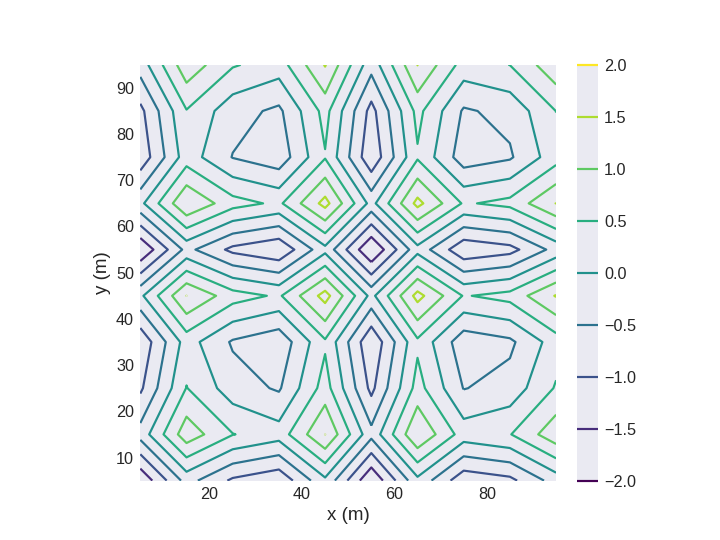
contour(ax=None, figsize=None, multiplier=None, filter_field=None, colorbar=True, colorbar_label=None, filename=None, **kwargs)

Contour line plot.

Before the field can be plotted, it must be sliced to give a plane (e.g. field.sel('z'), assuming field has three geometrical dimensions). In addition, field must be a scalar field (nvdim=1). Otherwise, ValueError is raised. mpl.contour adds the plot to matplotlib.axes.Axes passed via ax argument. If ax is not passed, matplotlib.axes.Axes object is created automatically and the size of a figure can be specified using figsize. By passing filter_field the points at which the pixels are not coloured can be determined. More precisely, only those discretisation cells where filter_field != 0 are plotted. Colorbar is shown by default and it can be removed from the plot by passing colorbar=False. The label for the colorbar can be defined by passing colorbar_label as a string.

It is often the case that the region size is small (e.g. on a nanoscale) or very large (e.g. in units of kilometers). Accordingly, multiplier can be passed as \(10^{n}\), where \(n\) is a multiple of 3 (…, -6, -3, 0, 3, 6,…). According to that value, the axes will be scaled and appropriate units shown. For instance, if multiplier=1e-9 is passed, all mesh points will be divided by \(1,\text{nm}\) and \(\text{nm}\) units will be used as axis labels. If multiplier is not passed, the best one is calculated internally. The plot can be saved as a PDF when filename is passed.

This method plots the field using matplotlib.pyplot.contour function, so any keyword arguments accepted by it can be passed (for instance, levels - number of levels, etc.).

Parameters:

• ax (matplotlib.axes.Axes, optional) – Axes to which the field plot is added. Defaults to None - axes are created internally.

• figsize ((2,) tuple, optional) – The size of a created figure if ax is not passed. Defaults to None.

• filter_field (discretisedfield.Field, optional) – A scalar field used for determining whether certain discretisation cells are coloured. More precisely, only those discretisation cells where filter_field != 0 are plotted. Defaults to None.

• colorbar (bool, optional) – If True, colorbar is shown and it is hidden when False. Defaults to True.

• colorbar_label (str, optional) – Colorbar label. Defaults to None.

• multiplier (numbers.Real, optional) – multiplier can be passed as \(10^{n}\), where \(n\) is a multiple of 3 (…, -6, -3, 0, 3, 6,…). According to that value, the axes will be scaled and appropriate units shown. For instance, if multiplier=1e-9 is passed, the mesh points will be divided by \(1\,\text{nm}\) and \(\text{nm}\) units will be used as axis labels. Defaults to None.

• filename (str, optional) – If filename is passed, the plot is saved. Defaults to None.

Raises:

ValueError – If the field has not 2D, its dimension is not 1, or the dimension of filter_field is not 1.

Example

1. Visualising the scalar field using matplotlib.

>>> import discretisedfield as df
>>> import math
...
>>> p1 = (0, 0, 0)
>>> p2 = (100, 100, 100)
>>> n = (10, 10, 10)
>>> mesh = df.Mesh(p1=p1, p2=p2, n=n)
>>> def init_value(point):
...     x, y, z = point
...     return math.sin(x) + math.sin(y)
>>> field = df.Field(mesh, nvdim=1, value=init_value)
>>> field.sel('z').mpl.contour()

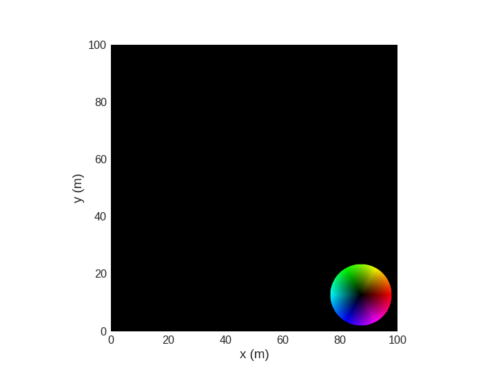
lightness(ax=None, figsize=None, multiplier=None, filter_field=None, lightness_field=None, clim=None, colorwheel=True, colorwheel_xlabel=None, colorwheel_ylabel=None, colorwheel_args=None, filename=None, **kwargs)

Lightness plots.

Uses HSV to show in-plane angle and lightness for out-of-plane (3d) or norm (1d/2d) of the field. By passing a scalar field as lightness_field, lightness component is can be specified independently of the field dimension. Most parameters are the same as for discretisedfield.plotting.Mpl.scalar. Colormap cannot be passed using kwargs. Instead of having a colorbar a colorwheel is displayed by default.

Parameters:

• lightness_field (discretisedfield.Field, optional) – A scalar field used for adding lightness to the color. Field values are hue. Defaults to None.

• colorwheel (bool, optional) – To control if a colorwheel is shown, defaults to True.

• colorwheel_xlabel (str, optional) – If specified, the string and an arrow are plotted onto the colorwheel (in x-direction).

• colorwheel_ylabel (str, optional) – If specified, the string and an arrow are plotted onto the colorwheel (in y-direction).

• colorwheel_args (dict, optional) – Additional keyword arguments to pass to the colorwheel function. For details see discretisedfield.plotting.Mpl.colorwheel and mpl_toolkits.axes_grid1.inset_locator.inset_axes.

Examples

1. Visualising the scalar field using matplotlib.

>>> import discretisedfield as df
...
>>> p1 = (0, 0, 0)
>>> p2 = (100, 100, 100)
>>> n = (10, 10, 10)
>>> mesh = df.Mesh(p1=p1, p2=p2, n=n)
>>> field = df.Field(mesh, nvdim=3, value=(1, 2, 3))
...
>>> field.sel('z').mpl.lightness()

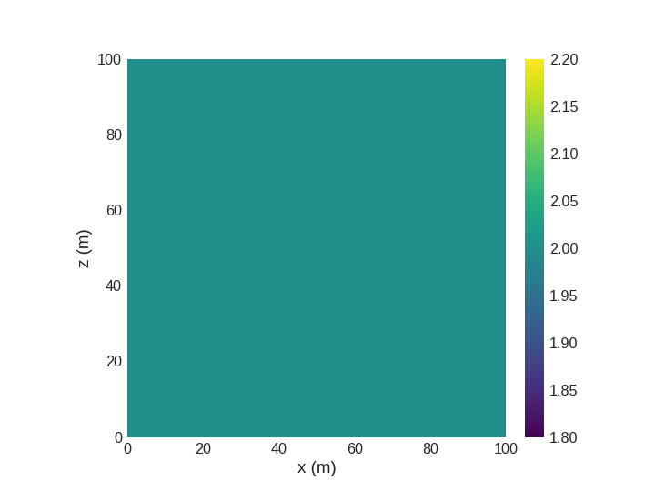
scalar(ax=None, figsize=None, multiplier=None, filter_field=None, colorbar=True, colorbar_label='', filename=None, symmetric_clim=False, **kwargs)

Plot the scalar field on a plane.

Before the field can be plotted, it must be sliced with a plane (e.g. field.sel('z'), assuming the geometry has three dimensions). In addition, field must be a scalar field (nvdim=1). Otherwise, ValueError is raised. mpl.scalar adds the plot to matplotlib.axes.Axes passed via ax argument. If ax is not passed, matplotlib.axes.Axes object is created automatically and the size of a figure can be specified using figsize. By passing filter_field the points at which the pixels are not coloured can be determined. More precisely, only those discretisation cells where filter_field != 0 are plotted. Colorbar is shown by default and it can be removed from the plot by passing colorbar=False. The label for the colorbar can be defined by passing colorbar_label as a string. If symmetric_clim=True is passed colorbar limits are internally computed to be symmetric around zero. This is most useful in combination with a diverging colormap. clim takes precedence over symmetric_clim if both are specified.

It is often the case that the region size is small (e.g. on a nanoscale) or very large (e.g. in units of kilometers). Accordingly, multiplier can be passed as \(10^{n}\), where \(n\) is a multiple of 3 (…, -6, -3, 0, 3, 6,…). According to that value, the axes will be scaled and appropriate units shown. For instance, if multiplier=1e-9 is passed, all mesh points will be divided by \(1\,\text{nm}\) and \(\text{nm}\) units will be used as axis labels. If multiplier is not passed, the best one is calculated internally. The plot can be saved as a PDF when filename is passed.

This method plots the field using matplotlib.pyplot.imshow function, so any keyword arguments accepted by it can be passed (for instance, cmap - colormap, clim - colorbar limits, etc.).

Parameters:

• ax (matplotlib.axes.Axes, optional) – Axes to which the field plot is added. Defaults to None - axes are created internally.

• figsize ((2,) tuple, optional) – The size of a created figure if ax is not passed. Defaults to None.

• filter_field (discretisedfield.Field, optional) – A scalar field used for determining whether certain discretisation cells are coloured. More precisely, only those discretisation cells where filter_field != 0 are plotted. Defaults to None.

• colorbar (bool, optional) – If True, colorbar is shown and it is hidden when False. Defaults to True.

• colorbar_label (str, optional) – Colorbar label. Defaults to None.

• symmetric_clim (bool, optional) – Automatic clim symmetric around 0. Defaults to False.

• multiplier (numbers.Real, optional) – multiplier can be passed as \(10^{n}\), where \(n\) is a multiple of 3 (…, -6, -3, 0, 3, 6,…). According to that value, the axes will be scaled and appropriate units shown. For instance, if multiplier=1e-9 is passed, the mesh points will be divided by \(1\\,\\text{nm}\) and \(\\text{nm}\) units will be used as axis labels. Defaults to None.

• filename (str, optional) – If filename is passed, the plot is saved. Defaults to None.

Raises:

ValueError – If the field has not been sliced, its dimension is not 1, or the dimension of filter_field is not 1.

Example

1. Visualising the scalar field using matplotlib.

>>> import discretisedfield as df
...
>>> p1 = (0, 0, 0)
>>> p2 = (100, 100, 100)
>>> n = (10, 10, 10)
>>> mesh = df.Mesh(p1=p1, p2=p2, n=n)
>>> field = df.Field(mesh, nvdim=1, value=2)
...
>>> field.sel('y').mpl.scalar()

See also

vector()

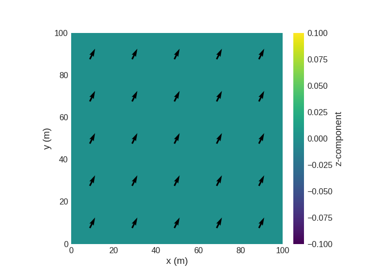
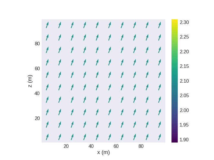
vector(ax=None, figsize=None, multiplier=None, vdims=None, use_color=True, color_field=None, colorbar=True, colorbar_label='', filename=None, **kwargs)

Plot the vector field on a plane.

Before the field can be plotted, it must be sliced to a plane (e.g. field.sel('z'), assuming the geometry has 3 dimensions). In addition, field must be a vector field of dimensionality two or three (i.e. nvdim=2 or nvdim=3). Otherwise, ValueError is raised. mpl.vector adds the plot to matplotlib.axes.axes passed via ax argument. If ax is not passed, matplotlib.axes.axes object is created automatically and the size of a figure can be specified using figsize. By default, plotted vectors are coloured according to the out-of-plane component of the vectors if the field has nvdim=3. This can be changed by passing color_field with nvdim=1. To disable colouring of the plot, use_color=False can be passed. A uniform vector colour can be obtained by specifying use_color=false and color=color which is passed to matplotlib. Colorbar is shown by default and it can be removed from the plot by passing colorbar=False. The label for the colorbar can be defined by passing colorbar_label as a string.

It is often the case that the region size is small (e.g. on a nanoscale) or very large (e.g. in units of kilometers). accordingly, multiplier can be passed as \(10^{n}\), where \(n\) is a multiple of 3 (…, -6, -3, 0, 3, 6,…). according to that value, the axes will be scaled and appropriate units shown. For instance, if multiplier=1e-9 is passed, all mesh points will be divided by \(1\,\text{nm}\) and \(\text{nm}\) units will be used as axis labels. If multiplier is not passed, the best one is calculated internally. The plot can be saved as a pdf when filename is passed.

This method plots the field using matplotlib.pyplot.quiver function, so any keyword arguments accepted by it can be passed (for instance, cmap - colormap, clim - colorbar limits, etc.). In particular, there are cases when matplotlib fails to find optimal scale for plotting vectors. More precisely, sometimes vectors appear too large in the plot. This can be resolved by passing scale argument, which scales all vectors in the plot. In other words, larger scale, smaller the vectors and vice versa. Please note that scale can be in a very large range (e.g. 1e20).

Parameters:

• ax (matplotlib.axes.axes, optional) – Axes to which the field plot is added. defaults to None - axes are created internally.

• figsize (tuple, optional) – The size of a created figure if ax is not passed. defaults to None.

• vdims (List[str], optional) – Names of the components to be used for the x and y component of the plotted arrows. This information is used to associate field components and spatial directions. Optionally, one of the list elements can be None if the field has no component in that direction. vdims is required for 2d vector fields.

• color_field (discretisedfield.field, optional) – A scalar field used for colouring the vectors. defaults to None and vectors are coloured according to their out-of-plane components.

• colorbar (bool, optional) – If true, colorbar is shown and it is hidden when false. defaults to true.

• colorbar_label (str, optional) – Colorbar label. Defaults to None.

• multiplier (numbers.real, optional) – multiplier can be passed as \(10^{n}\), where \(n\) is a multiple of 3 (…, -6, -3, 0, 3, 6,…). According to that value, the axes will be scaled and appropriate units shown. For instance, if multiplier=1e-9 is passed, the mesh points will be divided by \(1\,\text{nm}\) and \(\text{nm}\) units will be used as axis labels. defaults to None.

• filename (str, optional) – If filename is passed, the plot is saved. defaults to None.

Raises:

ValueError – If the field has not been sliced, its dimension is not 3, or the dimension of color_field is not 1.

Example

1. Visualising the vector field using matplotlib.

>>> import discretisedfield as df
...
>>> p1 = (0, 0, 0)
>>> p2 = (100, 100, 100)
>>> n = (10, 10, 10)
>>> mesh = df.Mesh(p1=p1, p2=p2, n=n)
>>> field = df.Field(mesh, nvdim=3, value=(1.1, 2.1, 3.1))
...
>>> field.sel('y').mpl.vector()

See also

mpl_scalar()