mag2exp.x_ray.holography

mag2exp.x_ray.holography(field, /, fwhm=None)

Calculation of the pattern obtained from X-ray holography.

X-ray holography uses magnetic circular dichroism to measure the magnetic field parallel to the propagation direction of the light. Here, we define the experimental reference frame with the light propagating along \(z\) direction. The results of X-ray holographic imaging is the real space integral of the magnetisation along the beam direction.

Parameters:

• field (discretisedfield.field) – Magnetisation field.

• fwhm (array_like, optional) – If specified, convolutes the output image with a 2 Dimensional Gaussian with the full width half maximum (fwhm) specified.

Returns:

X-ray holographic image.

Return type:

discretisedfield.Field

Examples

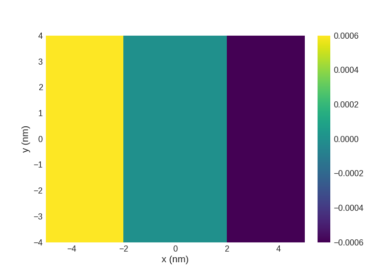
1. Visualising X-ray holography with matplotlib.

>>> import discretisedfield as df
>>> import mag2exp
>>> mesh = df.Mesh(p1=(-5e-9, -4e-9, 0), p2=(5e-9, 4e-9, 2e-9),
...                cell=(1e-9, 1e-9, 1e-9))
>>> def value_fun(point):
...     x, y, z = point
...     if x < -2e-9:
...         return (0, 0, 1)
...     elif x < 2e-9:
...         return (0, 1, 0)
...     else:
...         return (0, 0, -1)
>>> field = df.Field(mesh, nvdim=3, value=value_fun, norm=0.3e6)
>>> xrh = mag2exp.x_ray.holography(field)
>>> xrh.mpl.scalar()

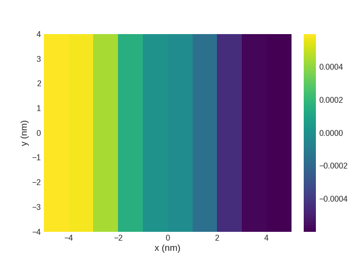
1. Visualising X-ray holography with matplotlib.

>>> import discretisedfield as df
>>> import mag2exp
>>> mesh = df.Mesh(p1=(-5e-9, -4e-9, 0), p2=(5e-9, 4e-9, 2e-9),
...                cell=(1e-9, 1e-9, 1e-9))
>>> def value_fun(point):
...     x, y, z = point
...     if x < -2e-9:
...         return (0, 0, 1)
...     elif x < 2e-9:
...         return (0, 1, 0)
...     else:
...         return (0, 0, -1)
>>> field = df.Field(mesh, nvdim=3, value=value_fun, norm=0.3e6)
>>> xrh2 = mag2exp.x_ray.holography(field, fwhm=(2e-9,2e-9))
>>> xrh2.mpl.scalar()