
mag2exp.ltem.defocus_image#
- mag2exp.ltem.defocus_image(phase, /, cs=0, df_length=0.0002, voltage=None, wavelength=None)#
Calculating the defocused image.
The wavefunction of the electrons is created from the magnetic phase shift \(\phi_m\)
\[\psi_0 = e^{i\phi_m},\]and propagated through the electron microscope to the image plane by use of the Contrast Transfer Function \(T\). The wavefunction at a defocus length \(\Delta f\) in Fourier space is given by
\[\widetilde{\psi}_{\Delta f} = \widetilde{\psi}_0 e^{2 i \pi \lambda k^2 (-\frac{1}{2} \Delta f + \frac{1}{4} C_s \lambda^2 k^2)},\]where \(\lambda\) is the relativistic wavelength of the electrons, \(C_s\) is the spherical aberration coefficient of the microscope, and \(k\) is the wavevector in Fourier space.
The intensity of an image at a specific defocus is given by
\[I_{\Delta f} = \left\vert \psi_{\Delta f} \right\vert^2.\]In focus \(I=\left\vert\psi_0\right\vert^2=1\)
Either electron
wavelengthor acceleration voltageUmust be specified.- Parameters:
phase (discretisedfield.Field) – Phase of the electrons from LTEM.
cs (numbers.Real, optional) – Spherical aberration coefficient.
df_length (numbers.Real, optional) – Defocus length in m.
voltage (numbers.Real, optional) – Accelerating voltage of electrons in V.
wavelength (numbers.Real, optional) – Relativistic wavelength of the electrons in m.
- Returns:
Intensity at specified defocus.
- Return type:
Examples
Zero defocus.
>>> import discretisedfield as df
>>> import mag2exp
>>> import numpy as np
>>> mesh = df.Mesh(p1=(-5e-9, -4e-9, -1e-9), p2=(5e-9, 4e-9, 1e-9),
...                    cell=(2e-9, 1e-9, 0.5e-9))
...
>>> def value_fun(point):
...     x, y, z = point
...     if x > 0:
...         return (0,-1, 0)
...     else:
...         return (0, 1, 0)
...
>>> field = df.Field(mesh, nvdim=3, value=value_fun)
>>> phase, ft_phase = mag2exp.ltem.phase(field)
>>> df_img = mag2exp.ltem.defocus_image(phase, cs=0, df_length=0,
...                                     voltage=300e3)
>>> np.allclose(df_img.array, [1])
True
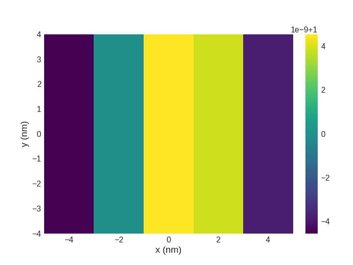
Visualising the phase using
matplotlib.
>>> import discretisedfield as df
>>> import mag2exp
>>> mesh = df.Mesh(p1=(-5e-9, -4e-9, -1e-9), p2=(5e-9, 4e-9, 1e-9),
...                    cell=(2e-9, 1e-9, 0.5e-9))
...
>>> def value_fun(point):
...     x, y, z = point
...     if x > 0:
...         return (0, -1, 0)
...     else:
...         return (0, 1, 0)
...
>>> field = df.Field(mesh, nvdim=3, value=value_fun)
>>> phase, ft_phase = mag2exp.ltem.phase(field)
>>> df_img = mag2exp.ltem.defocus_image(phase, cs=8000,
...                                     df_length=0.2e-3,
...                                     voltage=300e3)
>>> df_img.mpl.scalar()
See also